In this article we will have a look at an interesting Searching Algorithm: Interpolation Search. We will also look at some examples and the implementation. Along with this we look at complexity analysis of the algorithm and its advantage over other searching algorithms.
Interpolation Search is a modified or rather an improved variant of Binary Search Algorithm. This algorithm works on probing position of the required value to search, the search tries to get close to the actual value at every step or until the search item is found. Now, Interpolation search requires works on arrays with conditions:
- The Array should be Sorted in ascending order.
- The elements in the Array should have Uniform distribution. In other words, the difference between two successive elements (Arr[i] – Arr[i+1]) in the array for each pair must be equal.
Note: The second condition does not need to be true always. The given array cannot be fairly distributed sometimes. In that case, the probing index will help in search. We will look at the example for such case. The first condition has to be necessarily true.
In Binary Search, we used to get the index of our search element by dividing the array into two halves. So, We get the index of the middle element as mid = (low + high) / 2. If the index given by mid matches our key to search we return it, otherwise we search in the left or right half of the array depending on the value of mid.
Similarly, in the Interpolation search we get the index/position of the element based on a formula :
| Index = Low + ( ( (Key – Arr[Low]) * ( High – Low ) ) / Arr[High] -Arr[Low] ).
Let us look at each term: Arr: Sorted Array. Low: Index of first element in Array. High: Index of last element in Array. Key: Value to search. Note: The formula helps us get closer to the actual key by reducing number of steps. |
Interpolation Search Algorithm
- At first, We calculate the Index using the Interpolation probe position formula.
- Then, if the value at Index matches the key we search, simply return the index of the item and print the value at that index.
- If the item at the Index is not equal to key then we check if the Key is less than Arr[Index], calculate the probe position of the left sub-array by assigning High = Index – 1 and Low remains the same.
- If the Key is greater than Arr[Index], we calculate the Index for right subarray by assigning Low = Index + 1 and High remains same.
- We repeat these steps in a loop until the sub-array reduces to zero or until Low<=High.
Explanation with Examples
Now, let us understand how the algorithm helps in searching with some examples. There are mainly two cases to consider depending on input array.
Case 1: When Array is Uniformly Distributed
Now, let us look at an example how this formula gets us the index of the element. Consider this Array:
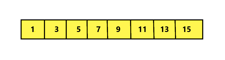
We can see the above array is sorted and is uniformly distributed in the sense that for each pair of element, e.g. 1 and 3 the difference is 2 and so is for every pair of elements in the array. Now let us assume we need to search for element 9 in the given array of size 8, we will use the above formula to get the index of the element 9.
Index = Low + ( ( (Key – Arr[Low]) * ( High – Low ) ) / Arr[High] -Arr[Low] ).
Here, Low = 0, High = Size – 1 = 8 – 1 = 7. Key = 9 and Arr[Low] = 1 and Arr[High] = 15.
So putting the values in the equation we get,
Index = 0 + ((9 – 1) * (7 – 0) / (15 – 1)) = 0 + ( 56 / 14 ) = 4.
Hence, we get the Index = 4 and at Arr[4] value is 9 and the value is found at index 4. So, we can see we found our key in only one step taking O(1) or Constant time without having the need to traverse the array. In Binary Search, it would have taken O(log n) time to find the key.
Case 2: When Array is Not Fairly/Uniformly Distributed
There might be a case when we will be given a sorted array which may not be fairly distributed i.e. the difference between two elements for each pair may not be equal. In such condition, we can search the value using Interpolation Search but the difference is the number of steps to get the index will increase. Let us consider understand this with an example.
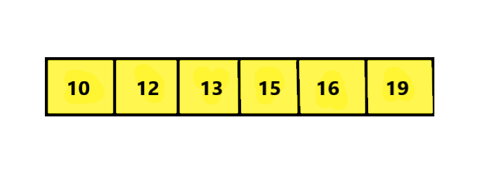
Here, we can see the above array is Sorted but not fairly distributed as the absolute difference between 10 and 12 is 2 whereas for 12 and 13 is 1, and for every pair the absolute difference is not equal. Now let’s say we want to search for element 13 in the given array of size 6. We will get the index using the Probing Position formula.
Index = Low + ( ( (Key – Arr[Low]) * ( High – Low ) ) / Arr[High] -Arr[Low] ).
Here, Low = 0, High = Size – 1 = 6 – 1 = 5. Key = 13 and Arr[Low] = 10 and Arr[High] = 19.
Now, putting the values we get,
Index = 0 + ((13 – 10) * (5 – 0)) / (19 – 10) = 0 + (3 * 5) / 9 = 15/9 = 1.66 ≈ 1 ( We approximate to Floor Value).
Now, Arr[Index] = Arr[1] = 12, so Arr[Index] < Key (13) , So we need to follow Step 4 of the Algorithm and we come to know that element exists in right subarray. Hence we assign Low = Index + 1 (1 + 1 = 2) and continue our search.
Hence, Low = 2, High = 5. Key = 13 and Arr[Low] = 13 and Arr[High] = 19.
So, Index = 2 + ((13 – 13) * (5 – 2)) / (19 – 13) = 2 + (0 * 3) / 9 = 2 + 0 = 2.
Now, At Index 2, Arr[Index] = 13 and we return the index of the element.
Implementation in Java
We will search for the element in the array and print the index considering 0 based indexing of array. We will consider both cases discussed above. Now, Let us look at the code for this:
|
1 2 3 4 5 6 7 8 9 10 11 12 13 14 15 16 17 18 19 20 21 22 23 24 25 26 27 28 29 30 31 32 33 34 35 36 37 38 39 40 41 42 43 44 45 46 47 48 49 50 51 52 53 54 55 56 57 58 59 60 61 62 63 64 65 66 |
import java.util.*; public class InterpolationSearch { static int interpolationSearch(int arr[], int low,int high, int key) { int index; while(low <= high) { // Calculating Exact Index or Closest Index to Key using Probing Position Formula. index = low + ( ( (key - arr[low]) * ( high - low ) ) / (arr[high] - arr[low])); // Condition when key is found if (arr[index] == key) return index; // If key is larger, key is in right sub array if (arr[index] < key) low = index + 1; // If key is smaller, key is in left sub array if (arr[index] > key) high = index - 1; } // if element does not exists we return -1. return -1; } public static void main(String args[]) { // We first perform search for a Sorted Uniformly Distributed Array -- Case 1 int arr[] = { 1, 3, 5, 7, 9, 11, 13, 15}; // Element to be searched int x = 9; int index = interpolationSearch(arr, 0, arr.length - 1, x); System.out.println("The Array is: "+Arrays.toString(arr)); // If element was found if (index != -1) System.out.println("Element "+x+" found at index: "+ index); else System.out.println("Element not found"); System.out.println(); // Then we perform search for Non-Uniformly Distibuted Array -- Case 2 arr = new int[]{10, 12, 13, 15, 16, 19}; // we search for value 13 x = 13; index = interpolationSearch(arr, 0, arr.length - 1, x); System.out.println("The Array is: "+Arrays.toString(arr)); // If element was found if (index != -1) System.out.println("Element "+x+" found at index: "+ index); else System.out.println("Element not found"); } } |
Output:
|
1 2 3 4 5 |
The Array is: [1, 3, 5, 7, 9, 11, 13, 15] Element 9 found at index: 4 The Array is: [10, 12, 13, 15, 16, 19] Element 13 found at index: 2 |
Time Complexity Analysis
Now, let us now quick look at the time complexity of the Interpolation Search Algorithm. There arise two cases when we consider the input array provided.
- Best Case: When the given array is Uniformly distributed, then the best case for this algorithm occurs which calculates the index of the search key in one step only taking constant or O(1) time.
- Average Case: If the array is not fairly distributed but sorted the average case occurs with runtime as O(log (log n)) in favorable situations, as we get close to the actual value’s index then we divide into subarrays. This is an improvisation over binary search algorithm which has O(log n) runtime.
So that’s it for the article you can try out the probing formula with different examples considering the two cases explained and execute the code for a better idea. Feel free to leave your suggestions/doubts in the comment section below.