


Credits
Hyperband: A novel bandit-based approach to hyperparameter optimization. — Li L, Jamieson K, DeSalvo G, Rostamizadeh A, Talwalkar A — JMLR 2018
This work has been done in collaboration with my colleague Simona Maggio (Check out her take on deep learning rate black magic here!).
Preliminaries
Explaining the inner working of Hyperband is beyond the reach of this blog post and we refer the reader to either the paper or the author’s blog post to fully understand the method. Yet, we introduce all the notations and variables required to understand our point.
Briefly, Hyperband is a method that aims to find the best hyperparameters for a model and a given budget. Following standard notations, we call a set of values for each parameter a configuration. Hyperband makes use of successive halving [2], a procedure that finds the best configuration among a set of randomly generated ones.
It finds the best configuration by iteratively training a model using each of them for a given budget, discarding the worst half, and repeating by doubling the budget until there is only one configuration left. Hyperband claims an optimal distribution of budget across several runs of successive halving to find a good enough solution both in cases where full exploration does best and where exploitation is useful.
For the rest of the blog post, we will focus on how Hyperband splits the budget among iterations of successive halving.
How the Budget Is Dispatched
Note: Since Medium does not support mathematical notations, we use superscript in the text in place of subscript.
Hyperband relies on two nested “for” loops. The outer loop iterates from 0 to 𝑠ᵐᵃˣ and runs a successive halving procedure each time. The successive halving inner loop, called a bracket, iterates 𝑠 times. It starts with 𝑛 models running with a budget 𝑟, and at each loop, the number of models is reduced by 𝜂 while the same factor increases the budget.
It is essential to understand that Hyperband splits the available budget equally between each of the outer loops, as specified in the paper on page seven:
Each bracket is designed to use approximately B total resources.
Let’s now have a look at the algorithm proposed in the paper. We’ve added the colored annotations that are not part of the original paper.
Within the algorithm:
- 𝜂, the pruning factor, is the factor of models eliminated at each bracket. For example, in the original successive halving procedure where 𝜂=2, one could start with 64 models, keep the best 32 models after the first bracket, then the best 16 models, and so on.
- 𝑛, in blue, is the number of models considered at each loop. Notice that the formula includes a division and a ceil operator to get an integer value. Following the preceding example, it would be 64.
- 𝑛ⁱ, in red, is the number of models used at iteration 𝑖. Notice that it is rounded using a floor operator.
- The unnamed quantity in green is the number of models kept from one iteration to the other. Again, it is rounded using a floor operator.
Since most of these values are rounded, we expect them to be fractions, not exact integers. The complicated formula for 𝑛 is designed to consume as much budget as possible at each Hyperband loop.
Discrepancy With the Example and Blog Post Implementation
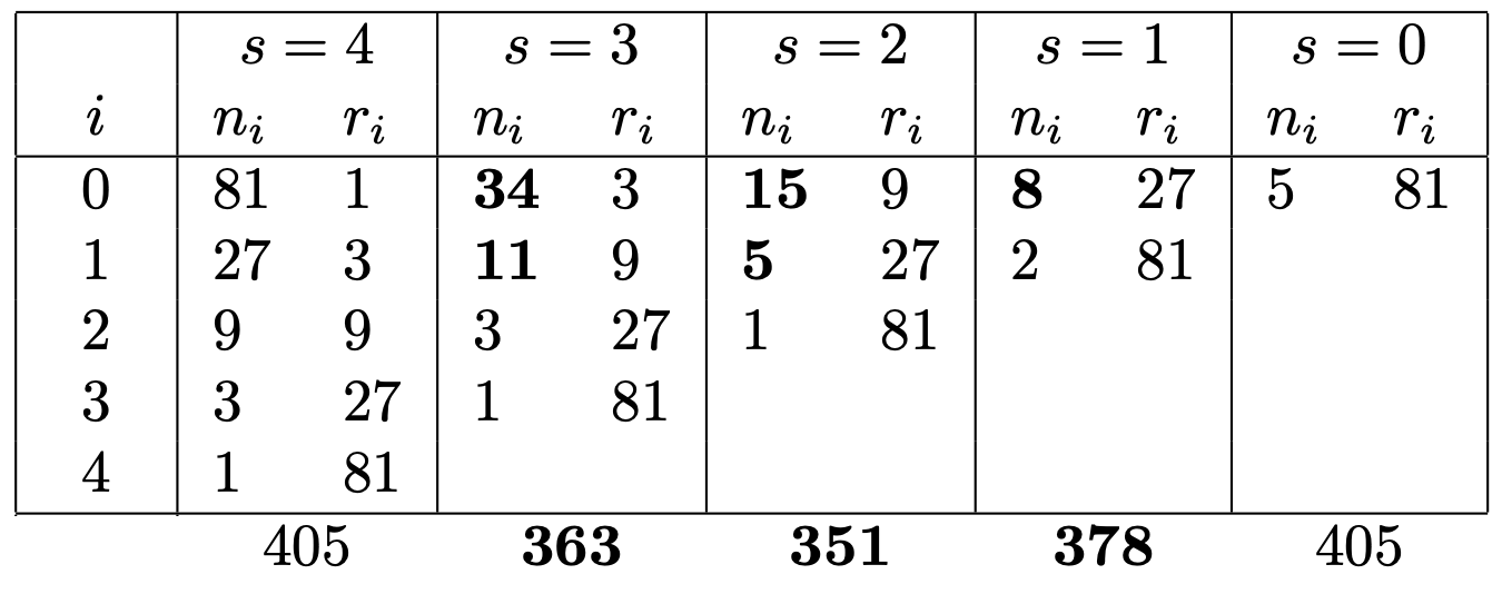
The paper provides a full example of how Hyperband splits its budget in Table 1. We have added the budget spent in each bracket in red.
We notice several things:
1. All values of 𝑛ⁱ are perfect multiples of powers of 𝜂 = 𝟑. This contradicts our previous intuition that these values could be fractional.
2. The budget can be as low as 243, which is nearly half of the budget of 405 allowed for each bracket. The total budget is 1,701, which is far from 2,025 allowed in this example.
The first observation stems from the implementation of Hyperband provided by the authors in a blog post [3] where the formula used to compute 𝑛 is written as:
n = int(ceil(int(B / max_iter / (s+1)) * eta ** s))
We recognize the ceiling operator. However, there is an additional rounding performed by the inner int casting. This rounding that is not present in the original formula enforces the values of 𝑛 to be perfect multiples of 𝜂.
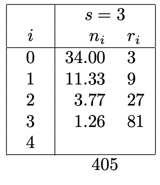
Let us remove this cast and compute what would be the same values in that case.
The total budget is now 1,902 which is closer to the ideal budget of 2,025. We can now justify the rounding operations present in the original algorithm. In fact, in the third column, we see that we start with 34 configurations and then go down to 11, whereas 34/3 = 11.33, hence the flooring operation. We believe that this table yields the results that were intended by the authors in the first place.
Most packages we could find implement the equation of the paper and therefore confirms our intuition:
- Keras Tuner
- Ray (see their comments about Hyperband implementation)
- Zygmuntz’s Hyperband
- Microsoft’s NNI
- Katib
- Harmonica
- Civis Analytics
While other packages opted for the code of the blog:
- HazyResearch and the associated PR
- HpBandSter and the associated PR
The story does not end here. Even in this configuration, some additional quick wins are easy to spot. For example, regarding the value of the 34 configurations evoked before, we notice that it is possible to start with 35 models instead of 34 without violating any constraints imposed in the paper. The cost of this bracket would then be 366, which is closer to our objective of 405.
Resource Allocation Is an Iterative Process
Why does the formula given in the paper fail to find this simple value? The reason lies in the non-rounded value. Let us compute the same column but without rounding the values.
Here, we see that the formula of the paper indeed gives us 34, but all the other values are not round. Computing the cost with the fractions sums up to 405. When adding another three-unit configuration, we implicitly borrow some budget unused during other iterations.
It highlights the inherent incremental nature of resource allocation: the budget not used during one iteration becomes available for the next one. We now use this property to devise a new resource allocator algorithm.
A Better Resource Allocator
Starting at this point, we will use a different approach than the one stated in the paper. Instead of trying to find a formula for 𝑛, we build it iteratively.
Our approach relies on natural intuition: budget spending. Instead of trying to find the best number 𝑛 of configurations directly, we simply compute the cost of adding one configuration in each successive iteration of the bracket and try to spend our budget the best way possible. There is indeed a cascading effect when adding a configuration to try: Adding a configuration at 𝑖=3 means that we need to add 𝜂 at the iteration 𝑖=2, and so on.
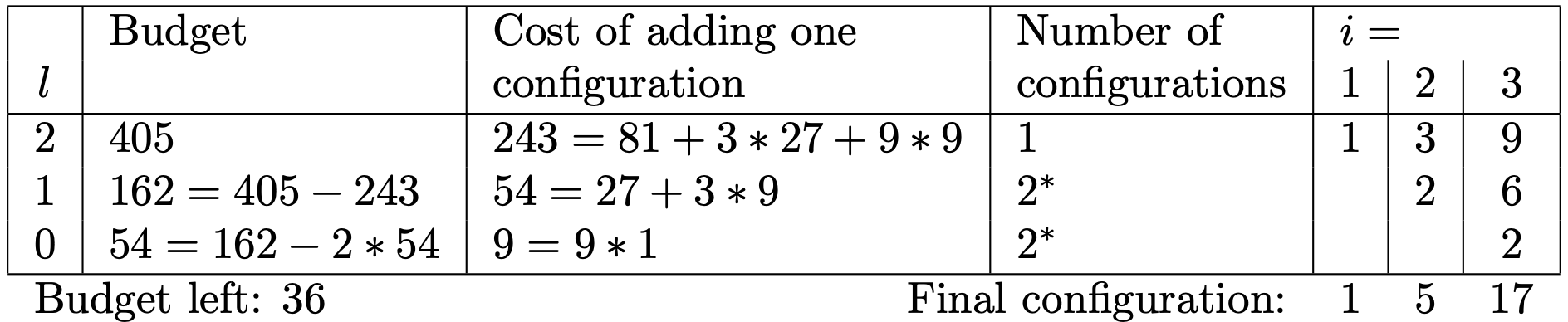
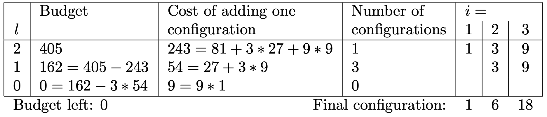
We build the budget for a bracket by considering the last iteration with the highest cost, adding as many configurations as possible without breaking the rule of maximum reduction factor of 𝜂, and then move to the next cheaper iteration. Here is an example of how to build a solution for bracket 𝑠=2 in our example. Note that we explore levels from 𝑙=2 (highest cost) to 𝑙=0:
See the code at the bottom of the post for more details. This approach is labelled as v1. Its application on the previous problem yields:
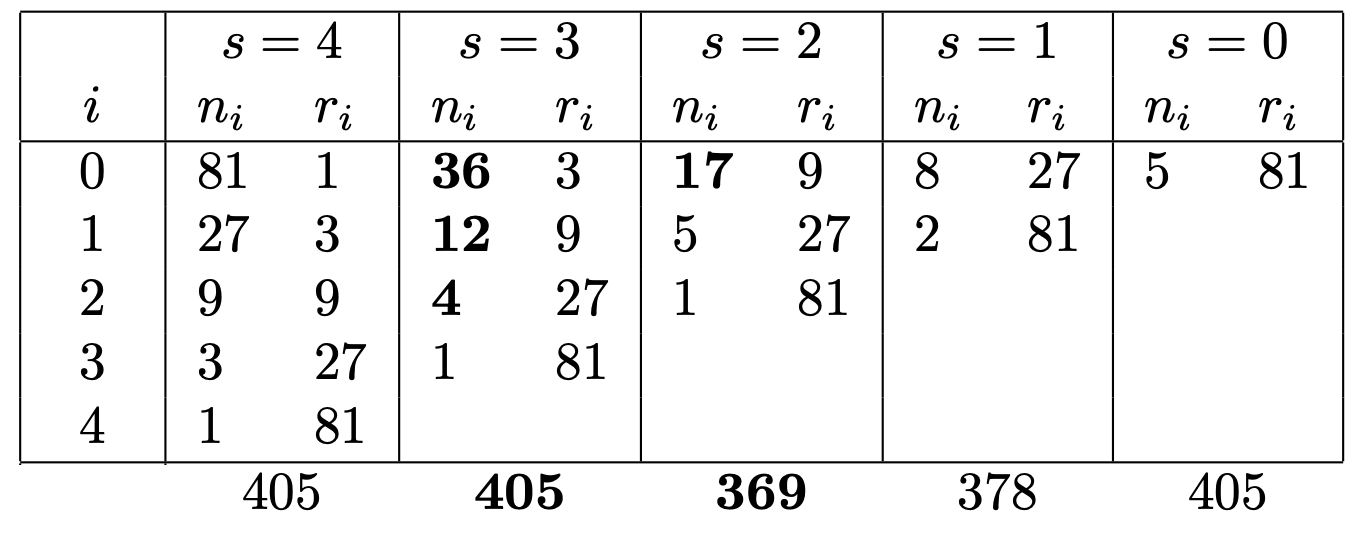
We now reach 405 for the second column, which is as far as we can go while respecting the constraints imposed in the paper. For this method, we have set up an explicit constraint to have the number of configurations reduced by the factor 𝜂. What happens if we lift this constraint?
Stepping Into the Illegal Zone
In this approach labeled as v2, we release the constraint of 𝜂 ratio between each successive halving iteration. We detail again the computation for bracket 𝑠=2:
Then, we apply it on the whole problem:

We have now maxed out the budget available in each bracket! It is even possible to do a bit better. Our current solution uses a budget of 2,025, respecting the maximum of 405 per bracket. We reach a perfect repartition just because the values of this example are convenient. However, it can happen that we still have some leftover budget at the end of a bracket.
In this case, as we have decided to allow the transfer of unused costs between one interaction of successive halving and the other, we can consider doing the same things across Hyperband iterations. The leftover budget of bracket s=0 would be transferred to the bracket s=1, and so on. However, the uplift brought by this strategy is minimal. We label it as v3.
Results Report and Still Existing Limitations
In order to compare methods, we look at the budget the authors use for all max_iter values between 11 and 277 — equivalent to 100 and 10,000 total budget. We report the score as a ratio compared to the ideal budget. The closer to one, the better.
Blog HB    0.8474179336338401
Paper HB   0.9283826113530446
Our HB v1  0.9710066977360124
Our HB v2  0.9973545216084753
Our HB v3  0.9999602719841088
Ideal      1.0000000000000000
These results confirm our findings on the simple example above. The blog implementation of Hyperband does not use 15% of the allocated budget, the paper version 7%, and our version only 3%. We also see that lifting some constraints can lead to near-perfect budget allocation.
Because most of the experiments are constrained by a fixed budget rather than a fixed number of max iterations for a given configuration, we look at the budget spent by each method with regards to the budget available.
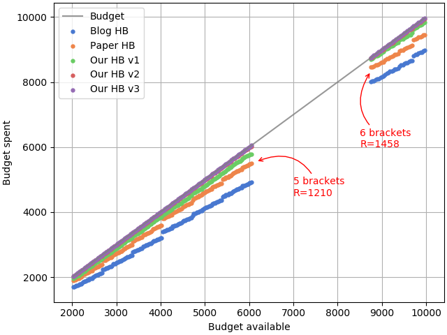
This figure shows how well the budget is used by each method compared to the ideal budget (grey line). The ranking of the methods is consistent with our previous observations.
One may notice the significant gaps present in the graph. They are caused by a sudden increase of total budget when the maximum iteration value causes the addition of a bracket:
- max_iter = 242 leads to 5 brackets of budget 1,210 for a total budget of 6,050
- max_iter = 243 leads to 6 brackets of budget 1,458 for a total budget of 8,748
This problem can be solved by giving a total budget to the function and computing the maximum resource per configuration from it. However, this changes the approach proposed by the authors completely, so we will not explore it further. It is important to note that when comparing methods by global budget, this budget should be outside of the blind spots of Hyperband.
Addendum: Of Bracket Count and 𝜂
The Ray Tune team reached out to us and pointed out that they had indeed noticed the discrepancy between the blog and paper formulae. They also had noticed the unexpected patterns in resource attribution. Everything is explained in their documentation.
In their study, they have focused on the total number of brackets executed rather than the global cost of the method. One of their finding is that changing the value of 𝜂 has also an unintuitive effect on the number of brackets:
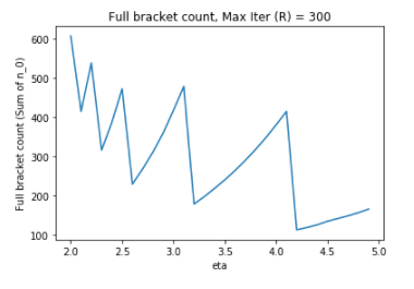
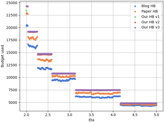
One may consequently wonders what is the impact of 𝜂 on the budget spent, if we keep max_iter fixed at 300. Here is the answer:
Conclusion
Here, we have shown that Hyperband can be tuned a little bit compared to the version found in the paper. We are still a bit surprised by the findings, but we could not find any resources discussing this discrepancy, knowing that several package maintainers decided willfully between the two implementations.
Finally, one unexpected advantage of the solution we propose here is that, as mentioned in the paper, the Hyperband computation proposed only works if it is not possible for the model to resume learning. Our proposed solution can be adapted to find the best budget with little effort in the case that resuming is, in fact, possible.
Big thanks to Léo for proofreading and making this post even better.