


Finding and Explaining Changes
Machine learning (ML) models deployed in production are usually paired with systems to monitor possible dataset drift. MLOps systems are designed to trigger alerts when drift is detected, but in order to make decisions about the strategy to follow next, we also need to understand what is actually changing in our data and what kind of abnormality the model is facing.
This post describes how to leverage a domain-discriminative classifier to identify the most atypical features and samples and shows how to use SHapley Additive exPlanations (SHAP) to boost the analysis of the data corruption.
 Atypical fall leaf
A Data Corruption Scenario
Aberrations can appear in incoming data for many reasons: noisy data collection, poorly performing sensors, data poisoning attacks, and more. These examples of data corruptions are a type of covariate shift that can be efficiently captured by drift detectors analyzing the feature distributions. For a refresher on dataset shift, have a look at this blog post.
Now, imagine being a data scientist working on the popular adult dataset, trying to predict whether a person earns over $50,000 a year, given their age, education, job, etc.
We train a predictor for this binary task on a random split of the dataset, constituting our source training set. We are happy with the trained model and deploy it in production together with a drift monitoring system.
The remaining part of the adult dataset represents the dataset provided at production time. Unfortunately, a part of this target-domain dataset is corrupted.
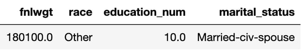 Figure 1: Constant values used to corrupt 25% of the target-domain samples
For illustration purposes, we poison 25% of the target-domain dataset, applying a constant replacement shift. This corrupts a random set of features, namely race, marital_status, fnlwgt, and education_num. The numeric features are corrupted by replacing their value with the median of the feature distribution, while the categorical features are corrupted by replacing their value with a fixed random category.
In this example, 25% of the target-domain samples have constant values for the four drifted features as shown in Figure 1. The drift detectors deployed to monitor data changes correctly trigger an alert. Now what?
How to Find the Most Drifted Samples?
A domain-discriminative classifier can rescue us. This secondary ML model, trained on half the source training set and half the new target-domain dataset, aims to predict whether a sample belongs to the Old Domain or the New Domain.
A domain classifier is actually a popular drift detector, as detailed here, thus the good news is that it’s not only good at detecting changes, but also at identifying atypical samples. If you already have a trained domain classifier in your monitoring system, you get a bonus novelty detector for free.
As a first guess, we can use the domain classifier probability score for the class New Domain as a drift score and highlight the top-k most atypical samples. But if there are hundreds of features, it is hard to make sense of the extracted top atypical samples. We need to narrow down the search by identifying the most drifted features.
In order to achieve this, we can for instance assume that the features most important for the domain discrimination are more correlated with the corruption. In this case, we can use a feature importance measure suitable for the domain classifier —for instance, a Mean Decrease of Impurity (MDI) for a random forest domain classifier.
There are many feature importance measures in the ML space and all have their own limitations. This is also one of the reasons why Shapley values have been introduced in the ML world through SHapley Additive exPlanations. For an introduction on the Shapley values and SHAP, have a look at the awesome Interpretable Machine Learning book.
Explaining the Drift
Using the SHAP package, we can explain the domain classifier outcome, specifically finding for a given sample how the different features contribute to the probability of belonging to the New domain. Looking at the Shapley values of the top atypical samples, we can thus understand what makes the domain classifier predict that a sample is indeed a novelty, thus uncovering the drifted features.
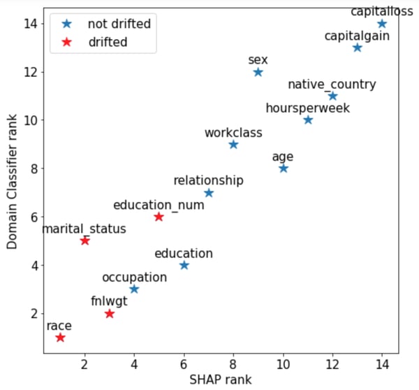 Figure 2: Comparison of importance ranks attributed to features: the lower the rank, the more drifted the feature is considered to be. The SHAP rank is based on average absolute Shapley values per feature in the whole test set. The domain classifier rank is given by the Mean Decrease of Impurity due to a feature.
In our adult dataset, in Figure 2 we compare the domain classifier feature importance and the SHAP feature importance (the average of all Shapley values in absolute value for a feature). We observe that they assign different ranks to the features, with SHAP correctly capturing the top-3 corrupted features. The choice of the importance measure has an impact on the identification of drifted features, thus it is essential to prefer techniques more reliable than the impurity criterion.
Instead of arbitrarily selecting the top-3 drifted features, one way of identifying drifted features is to compare the feature importance with a uniform importance (1/n_features) corresponding to undistinguishable domains. Then, we would spot the features that stand out, like in Figure 3 below, where race, marital_status and fnlwgt clearly show up.
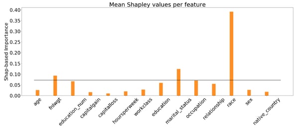 Figure 3. Average absolute Shapley values per feature in the target-domain dataset. Features with importance higher than the uniform importance (black line) are likely to be drifted.
If we plot the Shapley values for the entire target-domain dataset in Figure 4, highlighting all the true drifted samples in red, we can see that the Shapley values are quite expressive to find both the atypical samples and the atypical features. In each row of the summary plot, the same target-domain samples are represented as dots at the location of their Shapley values for a specific feature shown on the left. Here, we can observe the bimodal distributions for the atypical features selected previously (race, marital_status and fnlwgt), as well as for education_num, which is the last drifted feature to catch.
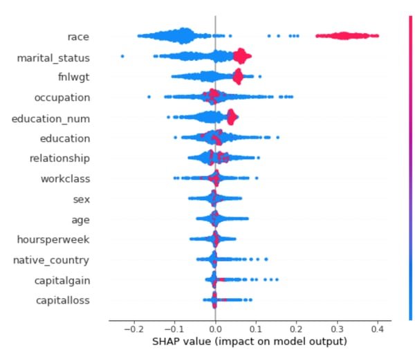 Figure 4: SHAP summary plot of the feature attribution for the target-domain samples. In each row, the same target-domain samples are represented as colored dots at the location of their Shapley values for a specific feature shown on the left. The color indicates whether the sample is truly atypical (red) or normal (blue).
By the efficiency property of the Shapley values, the domain classifier predicted score for a sample is the sum of its Shapley values for all the features. Thus, from the plot in Figure 4 above we can infer that the uncorrupted features have little (but non-zero) impact in predicting the New domain class, as their Shapley values are concentrated around zero, especially for the atypical samples (red dots).
Directly Visualizing the Drifted Samples
We’re ready now to wrap up and use those tools to actually highlight the suspicious samples and the atypical features.
First let’s have a look at the top-10 most atypical features and samples, as we could be lucky enough to perhaps visually understand what’s going on.
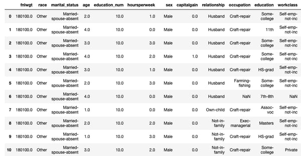 Figure 5: Top 10 most atypical samples according to the domain classifier probability score for the class New domain. Columns are sorted by the SHAP-based feature importance.
In this specific situation, we would probably recognize easily (and find suspicious) that all retrieved samples have constant values for some features, but this might not be the case in general. However, in some drift scenarios where the shift occurs at the distribution level, such as selection bias, looking at individual samples is not very useful. They would just be regular samples from a subpopulation of the source dataset, thus technically not an aberration. However, as we cannot know beforehand what kind of shift we are facing, it’s still a good idea to have a look at the individual samples !
A SHAP decision plot displaying the top-100 most atypical samples, like the one in Figure 6, where each curve represents one atypical sample, can help us see what is drifting. We also see it going towards higher domain classifier drift probabilities.
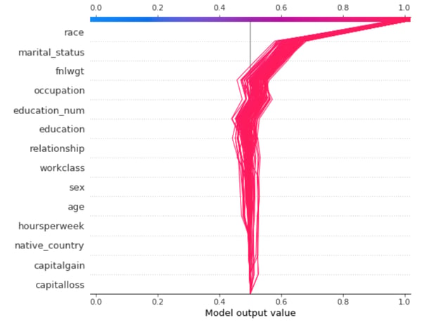 Figure 6: SHAP decision plot. Each curve represents one of the top 100 most atypical samples. The top features are the most contributing to make the sample atypical and 'pushing' the domain classifier probability for New domain towards higher values.
In this case, all the aberrations are due to the same corrupted features, but in the instance where groups of samples are drifting for different reasons, the SHAP decision plot would highlight these trends very efficiently.
Of course nothing can replace a standard analysis of feature distributions, especially now that we can select the most suspicious features to focus on. In Figure 7, we can look at the distribution of the drifted features for the top-100 atypical samples in red, and compare them with the baseline of samples from the source domain training set. As discriminative analysis is more intuitive for humans, this is a simple way to highlight what kind of drift is going on in the new dataset. In this example, looking at the feature distributions we can immediately spot that feature values are constant and don’t respect the expected distribution.
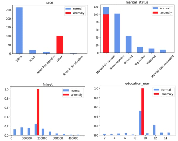 Figure 7: Distributions of the drifted features for the top 100 atypical samples (red) against the normal baseline (blue) from the source dataset.
Takeaways
When monitoring deployed models for unexpected data changes, we can take advantage of drift detectors, such as the domain classifier, to also identify atypical samples in case of drift alert. We can streamline the analysis of a drift scenario by highlighting the most drifted features to investigate. This selection can be done thanks to feature importance measures of the domain classifier.
Beware, though, of possible inconsistencies of feature importance measures and, if you can afford more computation, consider using SHAP for a more accurate drift-related relevance measure. Finally, combining useful SHAP visual tools with a discriminative analysis of drifted feature distributions with respect to the unshifted baseline will make your drift analysis simpler and more effective.