MCMC Methods: Metropolis-Hastings and Bayesian Inference
Markov Chain Monte Carlo (MCMC) methods let us compute samples from a distribution even though we can’t do this relying on traditional methods.
In this article, Toptal Data Scientist Divyanshu Kalra will introduce you to Bayesian methods and Metropolis-Hastings, demonstrating their potential in the field of probabilistic programming.

Divyanshu is a data scientist and full-stack developer versed in various languages. He has published three research papers in this field.
PREVIOUSLY AT

Let’s get the basic definition out of the way: Markov Chain Monte Carlo (MCMC) methods let us compute samples from a distribution even though we can’t compute it.
What does this mean? Let’s back up and talk about Monte Carlo Sampling.
Monte Carlo Sampling
What are Monte Carlo methods?
“Monte Carlo methods, or Monte Carlo experiments, are a broad class of computational algorithms that rely on repeated random sampling to obtain numerical results.” (Wikipedia)
Let’s break that down.
Example 1: Area Estimation
Imagine that you have an irregular shape, like the shape presented below:

And you are tasked with determining the area enclosed by this shape. One of the methods you can use is to make small squares in the shape, count the squares, and that will give you a pretty accurate approximation of the area. However, that is difficult and time-consuming.
Monte Carlo sampling to the rescue!
First, we draw a big square of a known area around the shape, for example of 50 cm2. Now we “hang” this square and start throwing darts randomly at the shape.

Next, we count the total number of darts in the rectangle and the number of darts in the shape we are interested in. Let’s assume that the total number of “darts” used was 100 and that 22 of them ended up within the shape. Now the area can be calculated by the simple formula:
area of shape = area of square *(number of darts in the shape) / (number of darts in the square)
So, in our case, this comes down to:
area of shape = 50 * 22/100 = 11 cm2
If we multiply the number of “darts” by a factor of 10, this approximation becomes very close to the real answer:
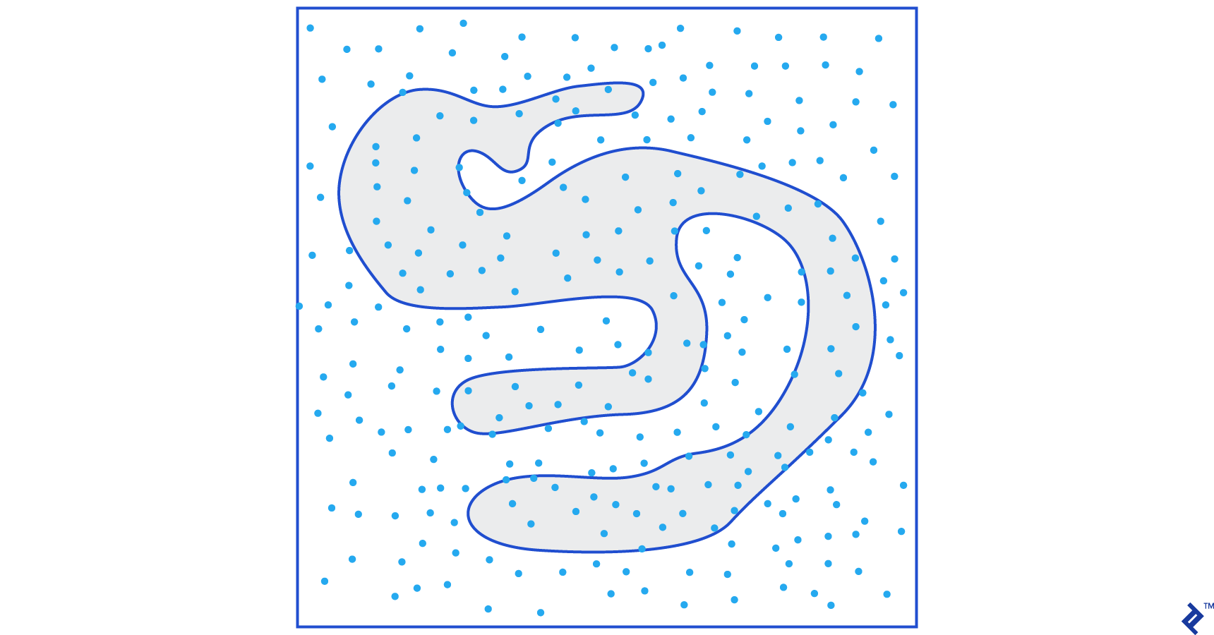
area of shape = 50 * 280/1000 = 14 cm2
This is how we break down complicated tasks, like the one given above, by using Monte Carlo sampling.
The Law of Large Numbers
The area approximation was closer the more darts we threw, and this is because of the Law of Large Numbers:
“The law of large numbers is a theorem that describes the result of performing the same experiment a large number of times. According to the law, the average of the results obtained from a large number of trials should be close to the expected value, and will tend to become closer as more trials are performed.”
This brings us to our next example, the famous Monty Hall problem.
Example 2: The Monty Hall Problem
The Monty Hall problem is a very famous brain teaser:
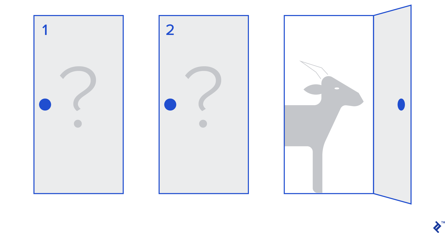
“There are three doors, one has a car behind it, the others have a goat behind them. You choose a door, the host opens a different door, and shows you there’s a goat behind it. He then asks you if you want to change your decision. Do you? Why? Why not?”
The first thing that comes to your mind is that the chances of winning are equal whether you switch or don’t, but that’s not true. Let’s make a simple flowchart to demonstrate the same.
Assuming that the car is behind door 3:

Hence, if you switch, you win ⅔ times, and if you don’t switch, you win only ⅓ times.
Let’s solve this by using sampling.
wins = []

for i in range(int(10e6)):

	car_door = assign_car_door()

	choice = random.randint(0, 2)

	opened_door = assign_door_to_open(car_door)

	did_he_win = win_or_lose(choice, car_door, opened_door, switch = False)

	wins.append(did_he_win)

print(sum(wins)/len(wins))
The assign_car_door() function is just a random number generator that selects a door 0, 1, or 2, behind which there is a car. Using assign_door_to_open selects a door that has a goat behind it and is not the one you selected, and the host opens it. win_or_lose returns true or false, denoting whether you won the car or not, it takes a bool “switch” which says whether you switched the door or not.
Let’s run this simulation 10 million times:
- Probability of winning if you don’t switch: 0.334134
- Probability of winning if you do switch: 0.667255
This is very close to the answers the flowchart gave us.
In fact, the more we run this simulation, the closer the answer comes to the true value, hence validating the law of large numbers:
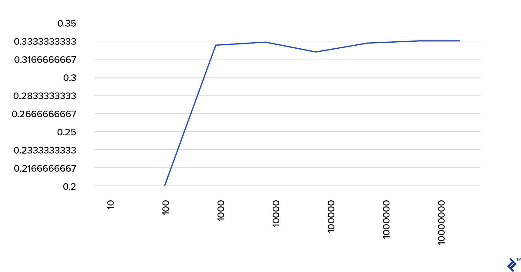
The same can be seen from this table:
| Simulations run | Probability of winning if you switch | Probability of winning if you don't switch |
| 10 | 0.6 | 0.2 |
| 10^2 | 0.63 | 0.33 |
| 10^3 | 0.661 | 0.333 |
| 10^4 | 0.6683 | 0.3236 |
| 10^5 | 0.66762 | 0.33171 |
| 10^6 | 0.667255 | 0.334134 |
| 10^7 | 0.6668756 | 0.3332821 |
The Bayesian Way of Thinking
“Frequentist, known as the more classical version of statistics, assume that probability is the long-run frequency of events (hence the bestowed title).”
“Bayesian statistics is a theory in the field of statistics based on the Bayesian interpretation of probability where probability expresses a degree of belief in an event. The degree of belief may be based on prior knowledge about the event, such as the results of previous experiments, or on personal beliefs about the event.” - from Probabilistic Programming and Bayesian Methods for Hackers
What does this mean?
In the frequentist way of thinking, we look at probabilities in the long run. When a frequentist says that there is a 0.001% chance of a car crash happening, it means, if we consider infinite car trips, 0.001% of them will end in a crash.
A Bayesian mindset is different, as we start with a prior, a belief. If we talk about a belief of 0, it means that your belief is that the event will never happen; conversely, a belief of 1 means that you are sure it will happen.
Then, once we start observing data, we update this belief to take into consideration the data. How do we do this? By using the Bayes theorem.
Bayes Theorem
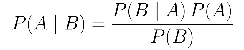
Let’s break it down.
-
P(A | B)gives us the probability of event A given event B. This is the posterior, B is the data we observed, so we are essentially saying what the probability of an event happening is, considering the data we observed. -
P(A)is the prior, our belief that event A will happen. -
P(B | A)is the likelihood, what is the probability that we will observe the data given that A is true.
Let’s look at an example, the cancer screening test.
Probability of Cancer
Let’s say a patient goes to get a mammogram done, and the mammogram comes back positive. What is the probability that the patient actually has cancer?
Let’s define the probabilities:
- 1% of women have breast cancer.
- Mammograms detect cancer 80% of the time when it is actually present.
- 9.6% of mammograms falsely report that you have cancer when you actually do not have it.
So, if you were to say that if a mammogram came back positive meaning there is an 80% chance that you have cancer, that would be wrong. You would not take into consideration that having cancer is a rare event, i.e., that only 1% of women have breast cancer. We need to take this as prior, and this is where the Bayes theorem comes into play:
P(C+ | T+) =(P(T+|C+)*P(C+))/P(T+)
-
P(C+ | T+): This is the probability that cancer is there, given that the test was positive, this is what we are interested in. -
P(T+ | C+): This is the probability that the test is positive, given that there is cancer, this, as discussed above is equal to 80% = 0.8. -
P(C+): This is the prior probability, the probability of an individual having cancer, which is equal to 1% = 0.01. -
P(T+): This is the probability that the test is positive, no matter what, so it has two components: P(T+) = P(T+|C-)P(C-)+P(T+|C+)P(C+) -
P(T+ | C-): This is the probability that the test came back positive but there is no cancer, this is given by 0.096. -
P(C-): This is the probability of not having cancer since the probability of having cancer is 1%, this is equal to 99% = 0.99. -
P(T+ | C+): This is the probability that the test came back positive, given that you have cancer, this is equal to 80% = 0.8. -
P(C+): This is the probability of having cancer, which is equal to 1% = 0.01.
Plugging all of this into the original formula:
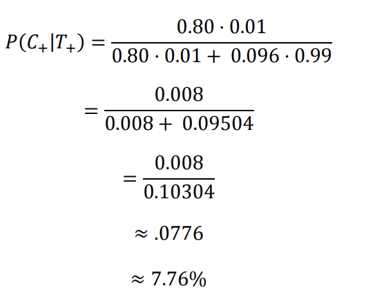
So, given that the mammogram came back positive, there is a 7.76% chance of the patient having cancer. It might seem strange at first but it makes sense. The test gives a false positive 9.6% of the time (quite high), so there will be many false positives in a given population. For a rare disease, most of the positive test results will be wrong.
Let us now revisit the Monty Hall problem and solve it using the Bayes theorem.
Monty Hall Problem
The priors can be defined as:
- Assume you choose door A as your choice in the beginning.
- P(H) = ⅓, ⅓. ⅓ for all three doors, which means that before the door was open and the goat revealed, there was an equal chance of the car being behind any of them.
The likelihood can be defined as:
-
P(D|H), where event D is that Monty chooses door B and there is no car behind it. -
P(D|H)= ½ if the car is behind door A - since there is a 50% chance that he will choose door B and 50% chance that he chooses door C. -
P(D|H)= 0 if the car is behind door B, since there is a 0% chance that he will choose door B if the car is behind it. -
P(D|H)= 1 if the car is behind C, and you choose A, there is a 100% probability that he will choose door B.
We are interested in P(H|D), which is the probability that the car is behind a door given that it shows us a goat behind one of the other doors.
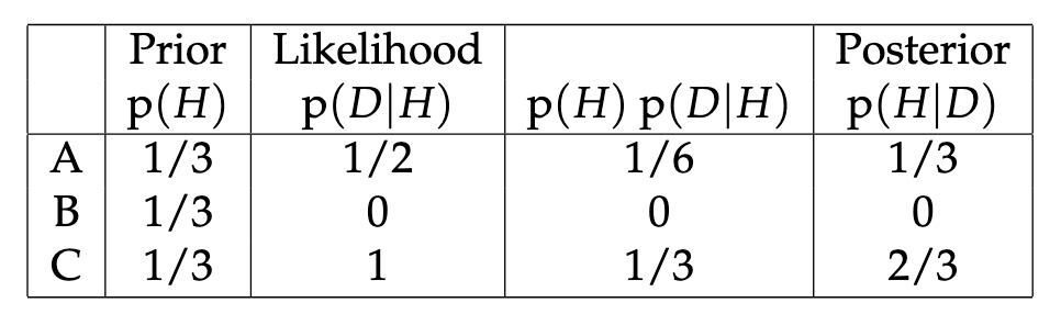
It can be seen from the posterior, P(H|D), that switching to door C from A will increase the probability of winning.
Metropolis-Hastings
Now, let’s combine everything we covered so far and try to understand how Metropolis-Hastings works.
Metropolis-Hastings uses the Bayes theorem to get the posterior distribution of a complex distribution, from which sampling directly is difficult.
How? Essentially, it randomly selects different samples from a space and checks if the new sample is more probable of being from the posterior than the last sample, since we are looking at the ratio of probabilities, P(B) in equation (1), gets canceled out:
P(acceptance) = ( P(newSample) * Likelihood of new sample) / (P(oldSample) * Likelihood of old sample)
The “likelihood” of each new sample is decided by the function f. That’s why f must be proportional to the posterior we want to sample from.
To decide if θ′ is to be accepted or rejected, the following ratio must be computed for each new proposed θ’:
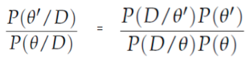
Where θ is the old sample, P(D| θ) is the likelihood of sample θ.
Let’s use an example to understand this better. Let’s say you have data but you want to find out the normal distribution that fits it, so:
X ~ N(mean, std)
Now we need to define the priors for the mean and std both. For simplicity, we will assume that both follow a normal distribution with mean 1 and std 2:
Mean ~ N(1, 2)
std ~ N(1, 2)
Now, let’s generate some data and assume the true mean and std are 0.5 and 1.2, respectively.
import numpy as np

import matplotlib.pyplot as plt

import scipy.stats as st

meanX = 1.5

stdX = 1.2

X = np.random.normal(meanX, stdX, size = 1000)

_ = plt.hist(X, bins = 50)
PyMC3
Let’s first use a library called PyMC3 to model the data and find the posterior distribution for the mean and std.
import pymc3 as pm

with pm.Model() as model:

  mean = pm.Normal("mean", mu = 1, sigma = 2)

  std = pm.Normal("std", mu = 1, sigma = 2)

  x = pm.Normal("X", mu = mean, sigma = std, observed = X)

  step = pm.Metropolis()

  trace = pm.sample(5000, step = step)
Let’s go over the code.
First, we define the prior for mean and std, i.e., a normal with mean 1 and std 2.
x = pm.Normal(“X”, mu = mean, sigma = std, observed = X)
In this line, we define the variable that we are interested in; it takes the mean and std we defined earlier, it also takes observed values that we calculated earlier.
Let’s look at the results:
_ = plt.hist(trace['std'], bins = 50, label = "std")

_ = plt.hist(trace['mean'], bins = 50, label = "mean")

_ = plt.legend()
The std is centered around 1.2, and the mean is at 1.55 - pretty close!
Let’s now do it from scratch to understand Metropolis-Hastings.
From Scratch
Generating a Proposal
First, let’s understand what Metropolis-Hastings does. Earlier in this article, we said, “Metropolis-Hastings randomly selects different samples from a space,” but how does it know which sample to select?
It does so using the proposal distribution. It is a normal distribution centered at the currently accepted sample and has an STD of 0.5. Where 0.5 is a hyperparameter, we can tweak; the more the STD of the proposal, the further it will search from the currently accepted sample. Let’s code this.
Since we have to find the mean and std of the distribution, this function will take the currently accepted mean and the currently accepted std, and return proposals for both.
def get_proposal(mean_current, std_current, proposal_width = 0.5):

    return np.random.normal(mean_current, proposal_width), \

            np.random.normal(std_current, proposal_width)
Accepting/Rejecting a Proposal
Now, let’s code the logic that accepts or rejects the proposal. It has two parts: the prior and the likelihood.
First, let’s calculate the probability of the proposal coming from the prior:
def prior(mean, std, prior_mean, prior_std):

        return st.norm(prior_mean[0], prior_mean[1]).pdf(mean)* \

                st.norm(prior_std[0], prior_std[1]).pdf(std)
It just takes the mean and std and calculates how likely it is that this mean and std came from the prior distribution that we defined.
In calculating the likelihood, we calculate how likely it is that the data that we saw came from the proposed distribution.
def likelihood(mean, std, data):

    return np.prod(st.norm(mean, std).pdf(X))
So for each data point, we multiply the probability of that data point coming from the proposed distribution.
Now, we need to call these functions for the current mean and std and for the proposed mean and std.
prior_current = prior(mean_current, std_current, prior_mean, prior_std)

likelihood_current = likelihood(mean_current, std_current, data)


prior_proposal = prior(mean_proposal, std_proposal, prior_mean, prior_std)

likelihood_proposal = likelihood(mean_proposal, std_proposal, data)
The whole code:
def accept_proposal(mean_proposal, std_proposal, mean_current, \

                    std_current, prior_mean, prior_std, data):


    def prior(mean, std, prior_mean, prior_std):

        return st.norm(prior_mean[0], prior_mean[1]).pdf(mean)* \

                st.norm(prior_std[0], prior_std[1]).pdf(std)


    def likelihood(mean, std, data):

        return np.prod(st.norm(mean, std).pdf(X))

    prior_current = prior(mean_current, std_current, prior_mean, prior_std)

    likelihood_current = likelihood(mean_current, std_current, data)


    prior_proposal = prior(mean_proposal, std_proposal, prior_mean, prior_std)

    likelihood_proposal = likelihood(mean_proposal, std_proposal, data)


    return (prior_proposal * likelihood_proposal) / (prior_current * likelihood_current)
Now, let’s create the final function that will tie everything together and generate the posterior samples we need.
Generating the Posterior
Now, we call the functions we have written above and generate the posterior!
def get_trace(data, samples = 5000):

    mean_prior = 1

    std_prior = 2


    mean_current = mean_prior

    std_current = std_prior


    trace = {

        "mean": [mean_current],

        "std": [std_current]

    }


    for i in tqdm(range(samples)):

        mean_proposal, std_proposal = get_proposal(mean_current, std_current)

        acceptance_prob = accept_proposal(mean_proposal, std_proposal, mean_current, \

                                         std_current, [mean_prior, std_prior], \

                                          [mean_prior, std_prior], data)

        if np.random.rand() < acceptance_prob:

            mean_current = mean_proposal

            std_current = std_proposal

        trace['mean'].append(mean_current)

        trace['std'].append(std_current)

    return trace
Room for Improvement
Log is your friend!
Recall a * b = antilog(log(a) + log(b)) and a / b = antilog(log(a) - log(b)).
This is beneficial to us because we will be dealing with very small probabilities, multiplying which will result in zero, so we will rather add the log prob, problem solved!
So, our previous code becomes:
def accept_proposal(mean_proposal, std_proposal, mean_current, \

                    std_current, prior_mean, prior_std, data):


    def prior(mean, std, prior_mean, prior_std):

        return st.norm(prior_mean[0], prior_mean[1]).logpdf(mean)+ \

                st.norm(prior_std[0], prior_std[1]).logpdf(std)


    def likelihood(mean, std, data):

        return np.sum(st.norm(mean, std).logpdf(X))

    prior_current = prior(mean_current, std_current, prior_mean, prior_std)

    likelihood_current = likelihood(mean_current, std_current, data)


    prior_proposal = prior(mean_proposal, std_proposal, prior_mean, prior_std)

    likelihood_proposal = likelihood(mean_proposal, std_proposal, data)


    return (prior_proposal + likelihood_proposal) - (prior_current + likelihood_current)
Since we are returning the log of probability of acceptance:
if np.random.rand() < acceptance_prob:
Becomes:
if math.log(np.random.rand()) < acceptance_prob:
Let’s run the new code and plot the results.
_ = plt.hist(trace['std'], bins = 50, label = "std")

_ = plt.hist(trace['mean'], bins = 50, label = "mean")

_ = plt.legend()
As you can see, the std is centered at 1.2, and the mean at 1.5. We did it!
Moving Forward
By now, you hopefully understand how Metropolis-Hastings works and you might be wondering where you can use it.
Well, Bayesian Methods for Hackers is an excellent book that explains probabilistic programming, and if you want to learn more about the Bayes theorem and its applications, Think Bayes is a great book by Allen B. Downey.
Thank you for reading, and I hope this article encourages you to discover the amazing world of Bayesian stats.
Understanding the basics
What does MCMC stand for?
MCMC stands for Markov Chain Monte Carlo, which is a class of methods for sampling from a probability distribution.
What is the Bayesian approach to decision-making?
In the Bayesian approach to decision-making, you first start with the prior, this is what your beliefs are, then as data comes in, you incorporate that data to update these priors to get the posterior.
What is a Bayesian model?
A Bayesian model is a statistical model where you use probability to represent all uncertainty within the model.
Divyanshu Kalra
Delhi, India
Member since October 30, 2017
About the author
Divyanshu is a data scientist and full-stack developer versed in various languages. He has published three research papers in this field.
PREVIOUSLY AT