


Recommendation engines are everywhere today, whether explicitly offered to users (e.g., Amazon or Netflix, the classic examples) or working behind the scenes to choose which content to surface without giving the user a choice. And while building a simple recommendation engine can be quite straightforward, the real challenge is to actually build one that works and where the business sees real uplift and value from its output.

Here, I’ll focus on the straightforward bit, presenting the main components of a recommendation engine project so that you can (hopefully) get the easy part out of the way and focus on the business value. Specifically, we’ll explore building a collaborative filtering recommender (both item- and user-based) and a content-based recommender.
We’ll work in SQL (Postgres flavor) and Python, and we’ll work with two generic datasets throughout the rest of this post:
- A visit dataset with format: user_id x product_id x visit
where visit is a binary indicator (1 if the user visited the product, 0 otherwise). But this could also be a rating in case of explicit feedback.
- A product description dataset with schema: product_id x description
Getting the Data Ready
When preparing data to use for a recommendation engine, the first thing to do is some normalization since you’ll need it for any of the recommendation scores — normalization will scale every score between 0 and 1 so that it’s possible to compare things against each other to understand what is a good recommendation and what’s not.
As the users and products often follow a long-tail distribution, we will also cut the long tail by filtering on users and products that occur frequently enough. You can see this part below:
WHERE b.nb_visit_product > 15 AND b.nb_visit_user > 5
The following SQL query will produce a table called visit_normalized with format:
product_id x user_id x nb_visit_user x nb_visit_product x visit_user_normed x visit_product_normed
SELECT
b."product_id",
b."user_id",
b."nb_visit_user",
b."nb_visit_product",
b."visit"/SQRT(SUM(b."visit"*b."visit")  OVER (PARTITION BY b."user_id")) AS visit_user_normed,
b."visit"/SQRT(SUM(b."visit"*b."visit")  OVER (PARTITION BY b."product_id")) AS visit_product_normed

FROM  (SELECT *,
              COUNT(*) OVER(PARTITION BY "user_id") as nb_visit_user,
              COUNT(*) OVER(PARTITION by "product_id") as nb_visit_product
        FROM "visit"
        ) as b
WHERE b.nb_visit_product > 15 AND b.nb_visit_user > 5
ORDER BY 1,2
Collaborative Filtering
There are two main types of collaborative filtering: user-based and item-based. Note that the two are entirely symmetric (or more precisely the transpose of each other). For both versions, we first need to compute a score of similarity between two users or between two products.
User-Based
Again, with user-based collaborative filtering, the key is to calculate a user similarity score. The following will produce a table user_similarity with format: user_1 x user_2 x similarity_user
SELECT c1."user_id" AS user_1,
       c2."user_id" AS user_2,
       SUM(c1."visit_user_normed"*c2."visit_user_normed") AS similarity_user

FROM "visit_normalized" c1
INNER JOIN "visit_normalized" c2
ON c1."product_id"=c2."product_id"

GROUP BY 1, 2
ORDER BY 1, 3 DESC
As there are usually too many pairs of users to score, we often restrict this query (cf. the condition WHERE b.rank <= 10) by limiting ourselves to the 10 highest user similarity scores per user. The table has then format user_1 x user_2 x similarity_user x rank and our query becomes:
SELECT b.*

    FROM(SELECT a.*,
       row_number() over(partition by a.user_1 order by a.similarity_user desc) as rank

       FROM(SELECT c1."user_id" AS user_1,
             c2."user_id" AS user_2,
             SUM(c1."visit_user_normed"*c2."visit_user_normed") AS similarity_user

           FROM "visit_normalized" c1
           INNER JOIN "visit_normalized" c2
           ON c1."product_id"=c2."product_id"

           GROUP BY 1, 2
           ORDER BY 1, 3 DESC) as a

    WHERE a.user_1 != a.user_2) as b

WHERE b.rank <= 10
We can then use this user similarity to score a product for a given user user_j :
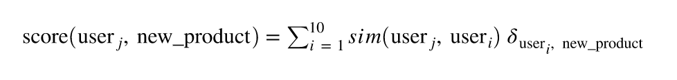
where 𝛿user, new_product (thanks Medium for this beautiful math rendering) is equal to 1 if the user has seen the new_product and 0 otherwise.
More generally, we could change 𝛿user, new_product by:
- The number of times user has seen the new product.
- The time spent by user on the new product.
- How long ago the user visited this product.
This is done using the following SQL script where the score_cf_user table will have the following format:
user_id x product_id x score_user_product
SELECT a.user_1 as user_id,
 b.product_id,
 SUM(a.similarity_user) as score_user_product

FROM user_similarity as a
INNER JOIN visit_normalised as b
ON a.user_2 = b.user_id

GROUP BY user_id,product_id
ORDER BY user_id,score_user_product DESC
Item-Based
We proceed similarly for the item-based collaborative filtering; we just need to transpose the above to produce the table product_similarity containing:
Product_1 x Product_2 x similarity_product
As usual, we restrict to the products that have been seen enough times (I chose 25, in this case — you can see below that this is done by the filtered_visit table).
with filtered_visit as (
SELECT *
FROM "visit_normalized"
WHERE nb_visit_product > 25
)

SELECT c1."product_id" AS Product_1,
       c2."product_id" AS Product_2,
       SUM(c1."visit_product_normed"*c2."visit_product_normed") AS similarity_product

FROM filtered_visit c1
INNER JOIN filtered_visit c2
ON c1."user_id"=c2."user_id"

GROUP BY 1, 2
ORDER BY 1, 3 DESC
And once again, we can then use this product similarity to score a product for a given user:

where 𝛿i, new_product is equal to 1 if the user has seen the new_product and 0 otherwise.
Again, let’s restrict the query to the 10 most similar products for a given product (cf. the condition WHERE final.rank <=10). The table score_cf_product has then format user_id x product_id x score_user_product x rank and our query becomes:
SELECT *
       FROM(
        SELECT *,
               row_number() over(partition by c."user_id" order by c.score_user_product desc) as rank
               FROM
                    (SELECT b."user_id",
                            a."product_2" as "product_id",
                            SUM(a."similarity_product") as score_user_product

                            FROM "product_similarity" as a
                            INNER JOIN "visit_normalized" as b
                            ON a."product_1" = b."product_id"
                            GROUP BY 1,2
                            ORDER BY 1,3 DESC
                    )as c
        )as final

WHERE final.rank <=10
Content-Based
With content-based recommendation engines, the overall philosophy is a bit different. Here, the goal is to use the description of the products to find products are similar to those that the user already bought or visited. To do that, we need a product classification, and we often have to build it from a text field. So that’s what we’ll walk through here.
TFIDF Version
We can describe each product by the (non-zero) term frequency–inverse document frequency (TFIDF) value of the words of its description.
The output dataset product_enriched_words has the following schema:
product_id x word x value
Given as follows:
from sklearn.feature_extraction.text import TfidfVectorizer, CountVectorizer
import pandas as pd
import time

##### TFIDF #####

# we suppose that ‘data’ is your product dataframe

data_samples=list(data['description'].fillna(' '))

print("Extracting tf-idf features for NMF...")
tfidf_vectorizer = TfidfVectorizer(max_df=0.95, min_df=2)
t0 = time()
tfidf = tfidf_vectorizer.fit_transform(data_samples)
print("done in %0.3fs." % (time() - t0))

##### CREATE WORD-VALUE DATASET #####

a=tfidf_vectorizer.inverse_transform(tfidf)
f=tfidf_vectorizer.get_feature_names()
tf=tfidf.toarray()
d={'product_id':[],'word':[],'value':[]}
list_book=list(data['product_id'])
for i in range(len(list_book)):
    list_word=list(a[i])
    for w in list_word:
        d['product_id'].append(list_book[i])
        d['word'].append(w)
        ind_=f.index(w)
        d['value'].append(tf[i][ind_])

product_enriched_words = pd.DataFrame(d)
By summing the product vectors seen by each user, we obtain the user profile:

This is done in with the following recipe whose output table user_profile_cb_words has format: user_id x word x value x value_normed
SELECT u."user_id", u."word", SUM(u."value") as value, SUM(u."value"*u."visit_product_normed") as value_normed
    FROM
        (SELECT w."product_id",w."value",w."word",b."user_id",b."visit_product_normed"
         FROM product_enriched_words w
        JOIN visit_normalized b
        ON w."product_id"=b."product_id") u
    GROUP BY u."user_id",u."word"
Finally, thanks to the user’s profile, we can score products :

(where <,> is your favorite scalar product)
This will give us the table score_cb_words with format: user_id x product_id x score_cb x score_cb_normed
SELECT a."user_id",a."product_id", SUM(a."score_cb") as score_cb, SUM(a."score_cb_normed") as score_cb_normed
       FROM
           (SELECT u."user_id",b."product_id", u."value"*b."value" as score_cb,
                   u."value_normed"*b."value" as score_cb_normed
            FROM user_profile_cb_words u
            JOIN product_enriched_words b
            ON u."word"=b."word") a
            GROUP BY a."user_id",a."product_id"
Non-Negative Matrix Factorization (NMF) Version
Another way to proceed on a content-based recommendation engine is to extract topics from the vector description. This allows for drastically reducing the dimension space, expressing each product by a vector of length n_topics.
Here, we present two versions of this method:
- A long format version for a direct SQL scoring
- A wide format version for a batch scoring in Python
Wide Format
This code is directly taken from the scikit-learn documentation. We only have to choose the number of desired topics, n_topics, and for displaying information about each topic, n_top_words.
The output dataset product_enriched_topics has format:
product_id x description x topic_0 x … x topic_9
##### TFIDF #####

# we suppose that ‘data’ is your ‘product’ dataframe

data_samples=list(data['description'].fillna(' '))

print("Extracting tf-idf features for NMF...")
tfidf_vectorizer = TfidfVectorizer(max_df=0.95, min_df=2)
t0 = time()
tfidf = tfidf_vectorizer.fit_transform(data_samples)
print("done in %0.3fs." % (time() - t0))

###### CREATE TOPIC DATASET WITH NMF #####

from sklearn.feature_extraction.text import TfidfVectorizer, CountVectorizer
from sklearn.decomposition import NMF

n_topics = 10
n_top_words = 5

def print_top_words(model, feature_names, n_top_words):
    for topic_idx, topic in enumerate(model.components_):
        print("Topic #%d:" % topic_idx)
        print(" ".join([feature_names[i]
                        for i in topic.argsort()[:-n_top_words - 1:-1]]))
    print()


print("Fitting the NMF model with tf-idf features")
t0 = time()
nmf = NMF(n_components=n_topics, random_state=1).fit(tfidf)
print("done in %0.3fs." % (time() - t0))

print("\nTopics in NMF model:")
tfidf_feature_names = tfidf_vectorizer.get_feature_names()
print_top_words(nmf, tfidf_feature_names, n_top_words)

res=pd.DataFrame(nmf.transform(tfidf))
res.columns=['topic'+str(i) for i in range(n_topics)]

product_enriched_topics = pd.concat([data,res],axis=1)
Like the TFIDF version, we can now deduce a user’s profile based on the NMF topics values. This first part computes the average topic values for each user, and the output table user_profile_cb has format:
user_id x topic0 x…x topic9 x topic0_normed x … x topic9_normed :
WITH user_product as
( SELECT 1 as value,
         b."user_id",
         AVG(t."topic0") as topic0 ,
         AVG(t."topic1") as topic1,
         AVG(t."topic2") as topic2,
         AVG(t."topic3") as topic3,
         AVG(t."topic4") as topic4,
         AVG(t."topic5") as topic5,
         AVG(t."topic6") as topic6,
         AVG(t."topic7") as topic7,
         AVG(t."topic8") as topic8,
         AVG(t."topic9") as topic9,

         AVG(t."topic0"*b."visit_product_normed") as topic0_normed,
         AVG(t."topic1"*b."visit_product_normed") as topic1_normed,
         AVG(t."topic2"*b."visit_product_normed") as topic2_normed,
         AVG(t."topic3"*b."visit_product_normed") as topic3_normed,
         AVG(t."topic4"*b."visit_product_normed") as topic4_normed,
         AVG(t."topic5"*b."visit_product_normed") as topic5_normed,
         AVG(t."topic6"*b."visit_product_normed") as topic6_normed,
         AVG(t."topic7"*b."visit_product_normed") as topic7_normed,
         AVG(t."topic8"*b."visit_product_normed") as topic8_normed,
         AVG(t."topic9"*b."visit_product_normed") as topic9_normed

 from visit_normalized b
 join product_enriched_topics t
 on b."product_id"=t."product_id"
 group by b."user_id")
Now, we can rescale those values by the average topic values over all users:
SELECT   t."user_id",
         t.topic0/AVG(t.topic0) over (partition by value) as topic0,
         t.topic1/AVG(t.topic1) over (partition by value) as topic1,
         t.topic2/AVG(t.topic2) over (partition by value) as topic2,
         t.topic3/AVG(t.topic3) over (partition by value) as topic3,
         t.topic4/AVG(t.topic4) over (partition by value) as topic4,
         t.topic5/AVG(t.topic5) over (partition by value) as topic5,
         t.topic6/AVG(t.topic6) over (partition by value) as topic6,
         t.topic7/AVG(t.topic7) over (partition by value) as topic7,
         t.topic8/AVG(t.topic8) over (partition by value) as topic8,
         t.topic9/AVG(t.topic9) over (partition by value) as topic9,

         t.topic0_normed/AVG(t.topic0_normed) over (partition by value) as topic0_normed,
         t.topic1_normed/AVG(t.topic1_normed) over (partition by value) as topic1_normed,
         t.topic2_normed/AVG(t.topic2_normed) over (partition by value) as topic2_normed,
         t.topic3_normed/AVG(t.topic3_normed) over (partition by value) as topic3_normed,
         t.topic4_normed/AVG(t.topic4_normed) over (partition by value) as topic4_normed,
         t.topic5_normed/AVG(t.topic5_normed) over (partition by value) as topic5_normed,
         t.topic6_normed/AVG(t.topic6_normed) over (partition by value) as topic6_normed,
         t.topic7_normed/AVG(t.topic7_normed) over (partition by value) as topic7_normed,
         t.topic8_normed/AVG(t.topic8_normed) over (partition by value) as topic8_normed,
         t.topic9_normed/AVG(t.topic9_normed) over (partition by value) as topic9_normed

 from user_product t
Finally, we can score new product in batch in Python with the following. The output dataset score_cb has then format:
user_id x product_id x score_cb x score_cb_normed
# we suppose that ‘product_to_score’ is your ‘product’ dataframe
# ‘user_profile_cb’ (we just computed it and we suppose you can access it via the path "file/to/user_profile_cb") will be read by batch

list_topic=['topic'+str(i) for i in range(10)]
list_topic_normed=['topic'+str(i)+'_normed' for i in range(10)]
list_topic_to_score=['topic'+str(i)+'_to_score' for i in range(10)]

def get_score(l):
    m=len(l)/2
    l1=l[0:m]
    l2=l[m:len(l)]
    return sum(np.array(l1)*np.array(l2))

#This function will be used to return the scalar product of the user's profile vector and the product's profile vector.

c=0
chunk_len=1000
product_to_score.columns=[x+'_to_score' for x in list(product_to_score.columns)]
product_to_score['key_']= 1

for df in pd.read_csv(“file/to/user_profile_cb”, chunksize = chunk_len, iterator = True):
    c=c+1
    print c*chunk_len
    df['key_']=1
    df=pd.merge(df,product_to_score,left_on='key_',right_on='key_')
    df['score_cb']=df[list_topic+list_topic_to_score].apply(lambda x: get_score(x),axis=1)
    df['score_cb_normed']=df[list_topic_normed+list_topic_to_score].apply(lambda x: get_score(x),axis=1)
    df=df[["user_id","product_id_to_score","score_cb","score_cb_normed"]]
    df.columns=["user_id","product_id","score_cb","score_cb_normed"]
    # You should know write df where you want (chunk by chunk)
Long Format
Starting from the NMF’s output product_enriched_topics, we can reshape this into a long format, product_enriched_topics_2, with schema: product_id x topic x value as follows:
v=list(product_enriched_topics.columns)
v.remove('description')
out2=out2[v]
out2=out2.set_index('product_id')
out2=out2.stack().reset_index()
out2.columns=['product_id','topic','value']

product_enriched_topics_2 = out2
As before, we can now easily compute the user profile and this gives us the table user_profile_cb_2 with format: user_id x topic x value x value_normed
SELECT u."user_id", u."topic",
         SUM(u."value") as value, SUM(u."value"*u."visit_product_normed") as value_normed
    FROM
        (SELECT w."product_id",w."value",w."topic",b."user_id",b."visit_product_normed"
        FROM product_enriched_topics_2 w
        JOIN visit_normalized b
        ON w."product_id"=b."product_id") u
   GROUP BY u."user_id",u."topic"
Last but not least, we can finally score in SQL:
SELECT a."user_id",a."product_id",
       SUM(a."score_cb") as score_cb, SUM(a."score_cb_normed") as score_cb_normed
FROM
       (SELECT u."user_id",b."product_id",
               u."value"*b."value" as score_cb, u."value_normed"*b."value" as score_cb_normed
        FROM user_profile_cb_2 u
        JOIN (SELECT * FROM product_enriched_topics_2 limit 100) b  --- to avoid memory error
              ON u."topic"=b."topic") a
                GROUP BY a."user_id",a."product_id"
Note that this may takes quite some time to run… but in the meantime — read on!
Mixing These Approaches — A Philosophy
We just saw how to compute several affinity scores, but you might be asking yourself: okay, which one do I take as my final result? Well, none of them, necessarily.
It’d be silly to arbitrarily choose one. We should instead be able to make some “average” of these different scores to compute our final affinity User/Product. How can we do that ?
The idea is to get the optimal combination between these scores. I’m sure it already rings a bell in your head… Yes, it’s a classical ML problem. We want to predict if a user will visit/buy/like a given product, and in order to do that we have a set of features which are the affinity scores we computed.
However, there will be one major difficulty: we only have positive examples to learn. Indeed, we always have the visits/buys/likes, but in many cases we don’t have the counterfactual events (didn’t visit/buy/like). This means that we will have to “create” those. This is what we call “negative sampling”.
Creating the Learning Set
The major difficulty in predicting if a user will visit/buy/like a given product is that we only have positive examples from which to learn. Indeed, we always have the visits, buys, and likes, but in many cases, we don’t have the counterfactual events (i.e., didn’t visit, didn’t buy, didn’t like).
This means that we will have to create those using what we call “negative sampling.” Imagine that you have your visit/buy user data until a given date T (which is probably today or yesterday). You will compute your several affinity scores by taking into account the data since a date T — x days, where x is a buffer you chose.
Then, you will be able to create a learning set with the data from T — x days until T. During this period of time, you have a set of User/Product couples that are “true” (i.e., the user bought the product during the period). But you don’t have negative examples, so you will have to create User/Product couples that are “false” (i.e., the user didn’t buy the product during the period). For each couple, your features will be the affinity scores you just computed, and the target will be “true” or “false." You try to find the best combination to optimize the visits, buys, and likes.
How many “false” couples should you create? Well, it’s a good question, and there is no real answer to this. It should be enough to have an unbalanced dataset, since in reality, the events visit, buy, or like are actually very unlikely to happen. How can I create «false» couples ? There are several strategies:
- Randomly (not a very good one).
- Randomly, but only picking users that visited, bought, or liked at least one thing during the period. We don’t pick users with only negative examples during that period because otherwise it would be too easy to have a good score, and it would not be very relevant.
- Excluding couples that happened in the past (if someone already bought something you don’t want to penalize it). We don’t take as fake example a true example from the past.
Now that your learning set is ready, you just have to split into a train and test set to create and evaluate your model. For the best possible results, you should do this split on a time basis.
Let’s say now that we have new columns date in our visit dataset:
user_id x product_id x visit x date
Here is the SQL code to create a learning set as described above with strategy number three:
SELECT f.*, 0 as target
FROM
 (	SELECT user_id, product_id
	FROM
	(SELECT distinct user_id
		FROM visit
		WHERE event_date > 'Your_Date_T - x days' and event_date < 'Your_Date_T')u,
	(SELECT distinct product_id FROM visit)p
	WHERE mod(user_id+product_id,20)
	)f
LEFT JOIN
(	SELECT distinct user_id,product_id,1 as real_
	FROM visit
	WHERE event_date > 'Your_Date_T - x days' and event_date < 'Your_Date_T'
	)r

ON f.user_id=r.user_id AND f.product_id=r.product_id
WHERE f.real_ is Null
UNION ALL
SELECT distinct user_id,product_id,1 as target
FROM visit
WHERE event_date > 'Your_Date_T - x days' and event_date < 'Your_Date_T'
Limitations
With the approach we’ve walked through here, note that once you trained a model based on your affinity scores, you will have to score all possible user/product couples. So obviously it can be extremely expensive if you have a huge catalog of products, which is why this approach better suits limited catalogs of products or content. We can think about ways to tackle this issue, but it will always mean limiting the set of available products (this limitation can be drawn by marketing rules, for example).
We also see that ultimately, the choice of the algorithm will be very important, because the scoring time will be completely different depending on this choice. A logistic regression could be a good choice in that case since it’s a linear combination which allows a really fast scoring.
So there you have it! You now have the basics with which to create a simple recommendation engine.