As kids, we learn a lot of things from our parents, but there is some information we get from our own experiences ‒ by unconsciously identifying patterns in our surroundings and applying them to new situations. In the world of artificial intelligence, that's how the unsupervised learning method works.
We’ve already touched on supervised learning. In this post, we’ll explain unsupervised learning – the other type of machine learning – its types, algorithms, use cases, and possible pitfalls.
What is unsupervised learning?
Unsupervised machine learning is the process of inferring underlying hidden patterns from historical data. Within such an approach, a machine learning model tries to find any similarities, differences, patterns, and structure in data by itself. No prior human intervention is needed.
Let's get back to our example of a child’s experiential learning.
Picture a toddler. The child knows what the family cat looks like (provided they have one) but has no idea that there are a lot of other cats in the world that are all different. The thing is, if the kid sees another cat, he or she will still be able to recognize it as a cat through a set of features such as two ears, four legs, a tail, fur, whiskers, etc.
In machine learning, this kind of prediction is called unsupervised learning. But when parents tell the child that the new animal is a cat – drumroll – that’s considered supervised learning.
Unsupervised learning finds a myriad of real-life applications, including:
data exploration,
customer segmentation,
recommender systems,
target marketing campaigns, and
data preparation and visualization, etc.
We'll cover use cases in more detail a bit later. As for now, let's grasp the essentials of unsupervised learning by comparing it to its cousin ‒ supervised learning.
Supervised learning vs unsupervised learning
The key difference is that with supervised learning, a model learns to predict outputs based on the labeled dataset, meaning it already contains the examples of correct answers carefully mapped out by human supervisors. Unsupervised learning, on the other hand, implies that a model swims in the ocean of unlabeled input data, trying to make sense of it without human supervision.
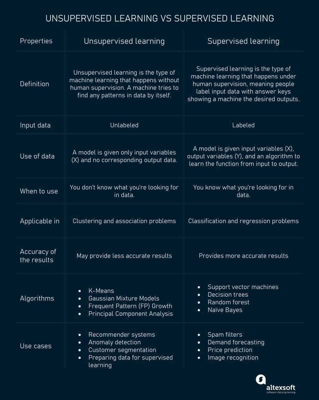
More differences between unsupervised vs supervised learning types are in the table below.
Unsupervised learning vs supervised learning
Now that we’ve compared the two approaches head to head, let’s move to the benefits brought to the table by unsupervised learning.
Why implement unsupervised machine learning?
While supervised learning has proved to be effective in various fields (e.g., sentiment analysis), unsupervised learning has the upper hand when it comes to raw data exploration needs.
Unsupervised learning is helpful for data science teams that don't know what they're looking for in data. It can be used to search for unknown similarities and differences in data and create corresponding groups. For example, user categorization by their social media activity.
The given method doesn't require training data to be labeled, saving time spent on manual classification tasks.
Unlabeled data is much easier and faster to get.
Such an approach can find unknown patterns and therefore useful insights in data that couldn’t be found otherwise.
It reduces the chance of human error and bias, which could occur during manual labeling processes.
Unsupervised learning can be approached through different techniques such as clustering, association rules, and dimensionality reduction. Let’s take a closer look at the working principles and use cases of each one.
Clustering algorithms: for anomaly detection and market segmentation
From all unsupervised learning techniques, clustering is surely the most commonly used one. This method groups similar data pieces into clusters that are not defined beforehand. An ML model finds any patterns, similarities, and/or differences within uncategorized data structure by itself. If any natural groups or classes exist in data, a model will be able to discover them.
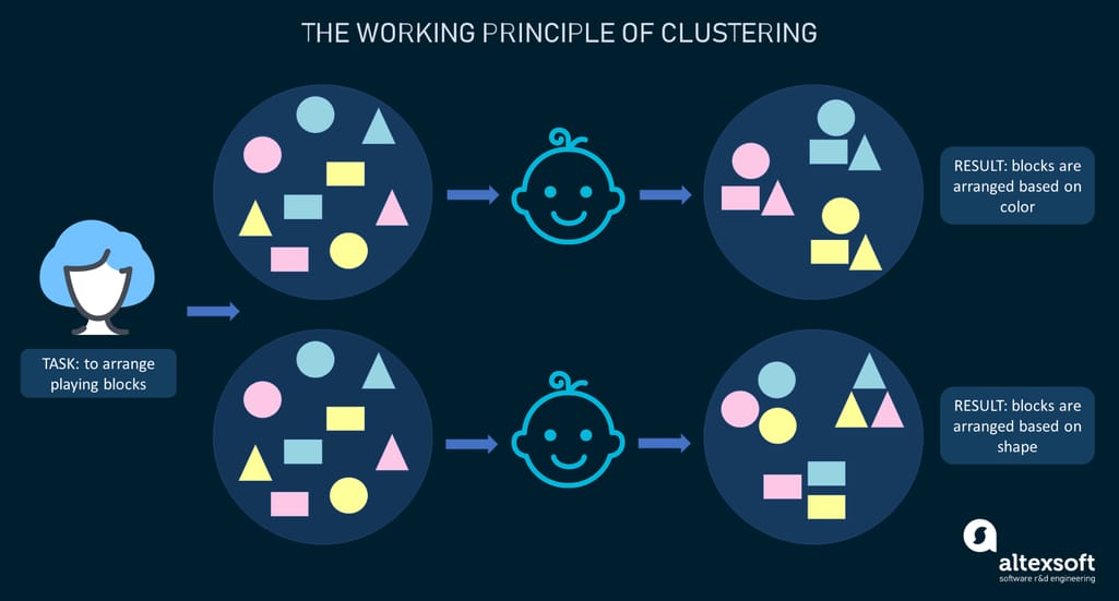
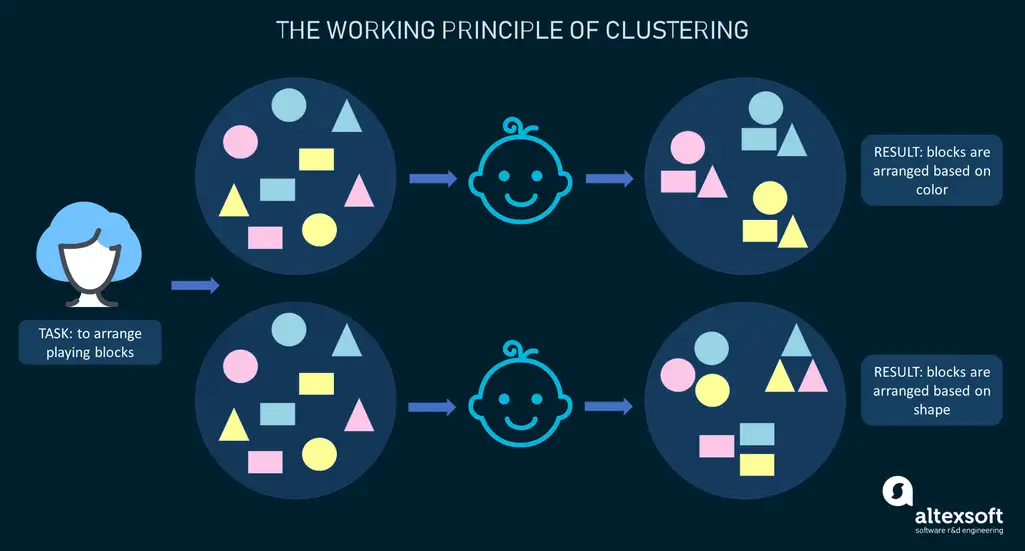
To explain the clustering approach, here's a simple analogy. In a kindergarten, a teacher asks children to arrange blocks of different shapes and colors. Suppose each child gets a set containing rectangular, triangular, and round blocks in yellow, blue, and pink.
Clustering explained with the example of the kindergarten arrangement task
The thing is a teacher hasn’t given the criteria on which the arrangement should be done so different children came up with different groupings. Some kids put all blocks into three clusters based on the color ‒ yellow, blue, and pink. Others categorized the same blocks based on their shape ‒ rectangular, triangular, and round. There is no right or wrong way to perform grouping as there was no task set in advance. That’s the whole beauty of clustering: It helps unfold various business insights you never knew were there.
Clustering examples and use cases
Thanks to the flexibility as well as the variety of available types and algorithms, clustering has various real-life applications. We’ll cover some of them below.
Anomaly detection. With clustering, it is possible to detect any sort of outliers in data. For example, companies engaged in transportation and logistics may use anomaly detection to identify logistical obstacles or expose defective mechanical parts (predictive maintenance). Financial organizations may utilize the technique to spot fraudulent transactions and react promptly, which ultimately can save lots of money. Check our video to learn more about detecting anomalies and fraud.
Fraud detection, explained
Customer and market segmentation. Clustering algorithms can help group people that have similar traits and create customer personas for more efficient marketing and targeting campaigns.
Clinical cancer studies. Machine learning and clustering methods are used to study cancer gene expression data (tissues) and predict cancer at early stages.
Clustering types
There is an array of clustering types that can be utilized. Let’s examine the main ones.
Exclusive clustering or “hard” clustering is the kind of grouping in which one piece of data can belong only to one cluster.
Overlapping clustering or “soft” clustering allows data items to be members of more than one cluster with different degrees of belonging. Additionally, probabilistic clustering may be used to solve “soft” clustering or density estimation issues and calculate the probability or likelihood of data points belonging to specific clusters.
Hierarchical clustering, aims, as the name suggests, at creating a hierarchy of clustered data items. To obtain clusters, data items are either decomposed or merged based on the hierarchy.
Of course, each clustering type relies on different algorithms and approaches to be conducted effectively.
K-means
K-means is an algorithm for exclusive clustering, also known as partitioning or segmentation. It puts the data points into the predefined number of clusters known as K. Basically, K in the K-means algorithm is the input since you tell the algorithm the number of clusters you want to identify in your data. Each data item then gets assigned to the nearest cluster center, called centroids (black dots in the picture). The latter act as data accumulation areas.
Ideal clustering with a single centroid in each cluster. Source: GeeksforGeeks
The procedure of clustering may be repeated several times until the clusters are well-defined.
Fuzzy K-means
Fuzzy K-means is an extension of the K-means algorithm used to perform overlapping clustering. Unlike the K-means algorithm, fuzzy K-means implies that data points can belong to more than one cluster with a certain level of closeness towards each.
Exclusive vs overlapping clustering example
The closeness is measured by the distance from a data point to the centroid of the cluster. So, sometimes there may be an overlap between different clusters.
Gaussian Mixture Models (GMMs)
Gaussian Mixture Models (GMMs) is an algorithm used in probabilistic clustering. Since the mean or variance is unknown, the models assume that there is a certain number of Gaussian distributions, each representing a separate cluster. The algorithm is basically utilized to decide which cluster a particular data point belongs to.
Hierarchical clustering
The hierarchical clustering approach may start with each data point assigned to a separate cluster. Two clusters that are closest to one another are then merged into a single cluster. The merging goes on iteratively till there's only one cluster left at the top. Such an approach is known as bottom-up or agglomerative.
The example shows how seven different clusters (data points) are merged step by step based on distance until they all create one large cluster.
In case you start with all data items attached to the same cluster and then perform splits until each data item is set as a separate cluster, the approach will be called top-down or divisive hierarchical clustering.
Association rules: for personalized recommender engines
An association rule is a rule-based unsupervised learning method aimed at discovering relationships and associations between different variables in large-scale datasets. The rules present how often a certain data item occurs in datasets and how strong and weak the connections between different objects are.
For example, a coffee shop sees that there are 100 customers on Saturday evening with 50 out of 100 of them buying cappuccino. Out of 50 customers who buy cappuccino, 25 also purchase a muffin. The association rule here is: If customers buy cappuccino, they will buy muffins too, with the support value of 25/100=25% and the confidence value of 25/50=50%. The support value indicates the popularity of a certain itemset in the whole dataset. The confidence value indicates the likelihood of item Y being purchased when item X is purchased.
Association rules examples and use cases
This technique is widely used to analyze customer purchasing habits, allowing companies to understand relationships between different products and build more effective business strategies.
Recommender systems. The association rules method is widely used to analyze buyer baskets and detect cross-category purchase correlations. A great example is Amazon’s “Frequently bought together” recommendations. The company aims to create more effective up-selling and cross-selling strategies and provide product suggestions based on the frequency of particular items to be found in one shopping cart.
How Amazon uses association rules in their marketing and sales
Say, if you decide to buy Dove body wash products on Amazon, you'll probably be offered to add some toothpaste and a set of toothbrushes to your cart because the algorithm calculated that these products are often purchased together by other customers.
Target marketing. Whatever the industry, the method of association rules can be used to extract rules to help build more effective target marketing strategies. For instance, a travel agency may use customer demographic information as well as historical data about previous campaigns to decide on the groups of clients they should target for their new marketing campaign.
Let’s take a look at this paper published by Canadian travel and tourism researchers. Thanks to the use of association rules, they managed to single out sets of travel activity combinations that particular groups of tourists are likely to be involved in based on their nationality. They discovered that Japanese tourists tended to visit historic sites or amusement parks while US travelers would prefer attending a festival or fair and a cultural performance.
Among various algorithms applied to create association rules, apriori and frequent pattern (FP) growth are the most commonly used ones.
Apriori and FP-Growth algorithms
The apriori algorithm utilizes frequent itemsets to create association rules. Frequent itemsets are the items with a greater value of support. The algorithm generates the itemsets and finds associations by performing multiple scanning of the full dataset. Say, you have four transactions:
transaction 1={apple, peach, grapes, banana};
transaction 2={apple, potato, tomato, banana};
transaction 3={apple, cucumber, onion}; and
transaction 4={oranges, grapes}.
How frequent itemsets are singled out in the transactions
As we can see from the transactions, the frequent itemsets are {apple}, {grapes}, and {banana} according to the calculated support value of each. Itemsets can contain multiple items. For instance, the support value for {apple, banana} is two out four, or 50%.
Just like apriori, the frequent pattern growth algorithm also generates the frequent itemsets and mines association rules, but it doesn't go through the complete dataset several times. The users themselves define the minimum support for a particular itemset.
Dimensionality reduction: for effective data preparation
Dimensionality reduction is another type of unsupervised learning pulling a set of methods to reduce the number of features - or dimensions - in a dataset. Let us explain.
When preparing your dataset for machine learning, it may be quite tempting to include as much data as possible. Don’t get us wrong, this approach works well as in most cases more data means more accurate results.
Data preparation, explained
That said, imagine that data resides in the N-dimensional space with each feature representing a separate dimension. A lot of data means there may be hundreds of dimensions. Think of Excel spreadsheets with columns serving as features and rows as data points. Sometimes, the number of dimensions gets too high, resulting in the performance reduction of ML algorithms and data visualization hindering. So, it makes sense to reduce the number of features – or dimensions – and include only relevant data. That’s what dimensionality reduction is. With it, the number of data inputs becomes manageable while the integrity of the dataset isn't lost.
Dimensionality reduction use cases
The dimensionality reduction technique can be applied during the stage of data preparation for supervised machine learning. With it, it is possible to get rid of redundant and junk data, leaving those items that are the most relevant for a project.
Say, you work in a hotel and you need to predict customer demand for different types of hotel rooms. There’s a large dataset with customer demographics and information on how many times each customer booked a particular hotel room last year. It looks like this:
A small snapshot of columns and rows from a dataset
The thing is, some of this information may be useless for your prediction, while some data has quite a lot of overlap and there's no need to consider it individually. Take a closer look and you'll see that all customers come from the US, meaning that this feature has zero variance and can be removed. Since room service breakfast is offered with all room types, the feature also won't make much impact on your prediction. Features like "age" and "date of birth" can be merged as they are basically duplicates. So, in this way, you perform dimensionality reduction and make your dataset smaller and more useful.
Principal Component Analysis algorithm
Principal component analysis is an algorithm applied for dimensionality reduction purposes. It’s used to reduce the number of features within large datasets, which leads to the increased simplicity of data without the loss of its accuracy. Dataset compression happens through the process called feature extraction. It means that features within the original set are combined into a new, smaller one. Such new features are known as principal components.
Of course, there are other algorithms to apply in your unsupervised learning projects. The ones above are just the most common, which is why they are covered more thoroughly.
Unsupervised learning pitfalls to be aware of
As we can see from the post, unsupervised learning is attractive in lots of ways: starting with the opportunities to discover useful insights in data all the way to the elimination of expensive data labeling processes. But this approach to train machine learning models also has pitfalls you need to be aware of. Here are some of them.
The results provided by unsupervised learning models may be less accurate as input data doesn't contain labels as answer keys.
The method requires output validation by humans, internal or external experts who know the field of research.
The training process is relatively time-consuming because algorithms need to analyze and calculate all existing possibilities.
More often than not unsupervised learning deals with huge datasets which may increase the computational complexity.
Despite these pitfalls, unsupervised machine learning is a robust tool in the hands of data scientists, data engineers, and machine learning engineers as it is capable of bringing any business of any industry to a whole new level.