Processing one billion events per second with NiFi

Ever wonder how fast Apache NiFi is?

Ever wonder how well NiFi scales?

A single NiFi cluster can process trillions of events and petabytes of data per day with full data provenance and lineage. Here’s how.

When a customer is looking to use NiFi in a production environment, these are usually among the first questions asked. They want to know how much hardware they will need, and whether or not NiFi can accommodate their data rates.

This isn’t surprising. Today’s world consists of ever-increasing data volumes. Users need tools that make it easy to handle these data rates. If even one of the tools in an enterprise’s stack is not able to keep up with the data rate needed, the enterprise will have a bottleneck that prevents the rest of the tools from accessing the data they need.

NiFi performs a large variety of tasks and operates on data of all types and sizes. This makes it challenging to say how much hardware will be needed without fully understanding the use case. If NiFi is only responsible for moving data from an FTP server to HDFS, it will need few resources. If NiFi is responsible for ingesting data from hundreds of sources, filtering, routing, performing complex transformations, and finally delivering the data to several different destinations, it will require additional resources.

Fortunately, the answer to the latter question – Can NiFi scale to the degree that I need? – is much simpler. The answer is almost always a resounding “Yes!” In this article, we define a common use case and demonstrate how NiFi achieves both high scalability and performance for a real-world data processing scenario.

Use Case

Before diving into numbers and statistics, it is important to understand the use case. An ideal use case is one that is realistic yet simple enough that it can be explained concisely.

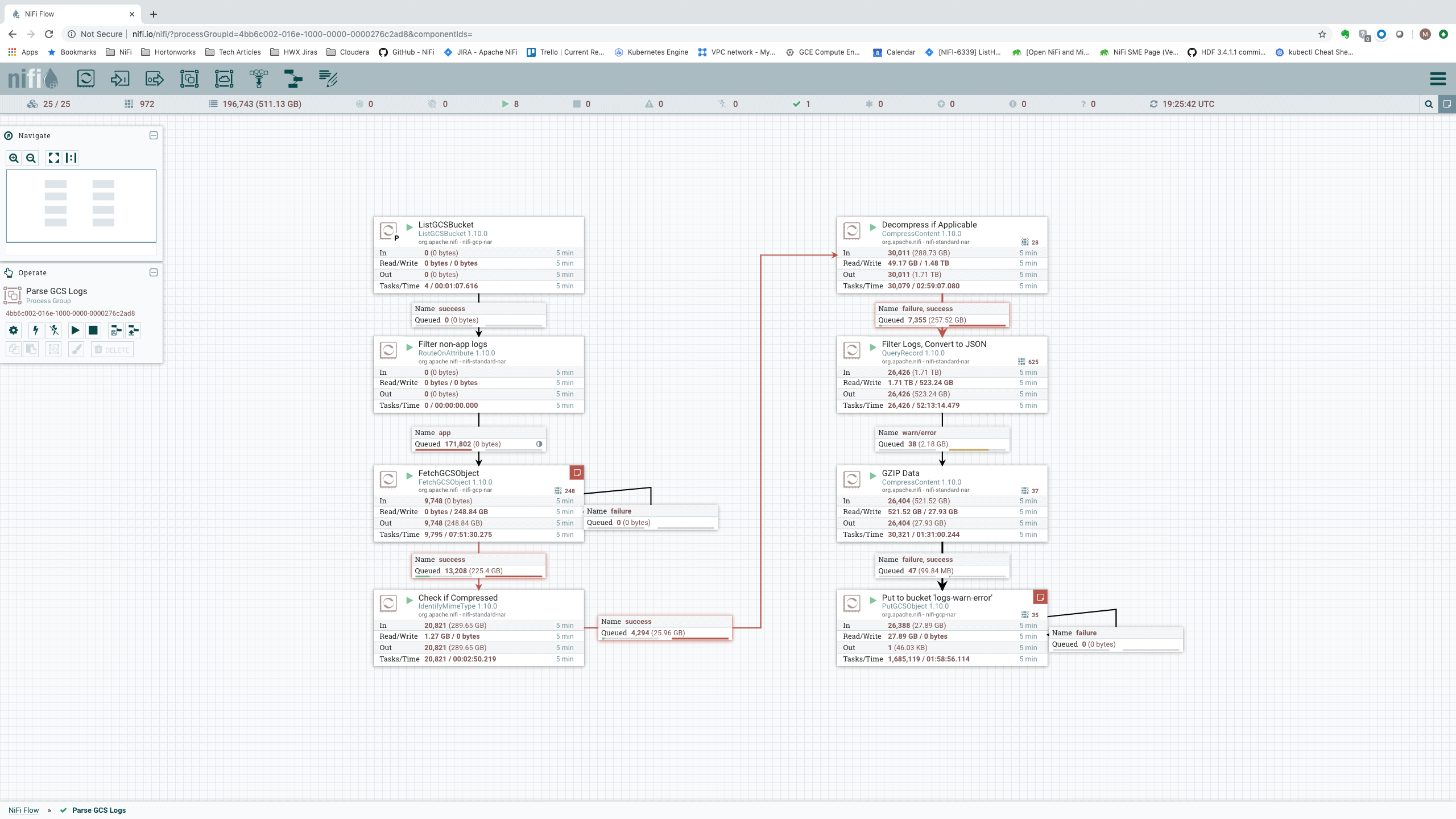
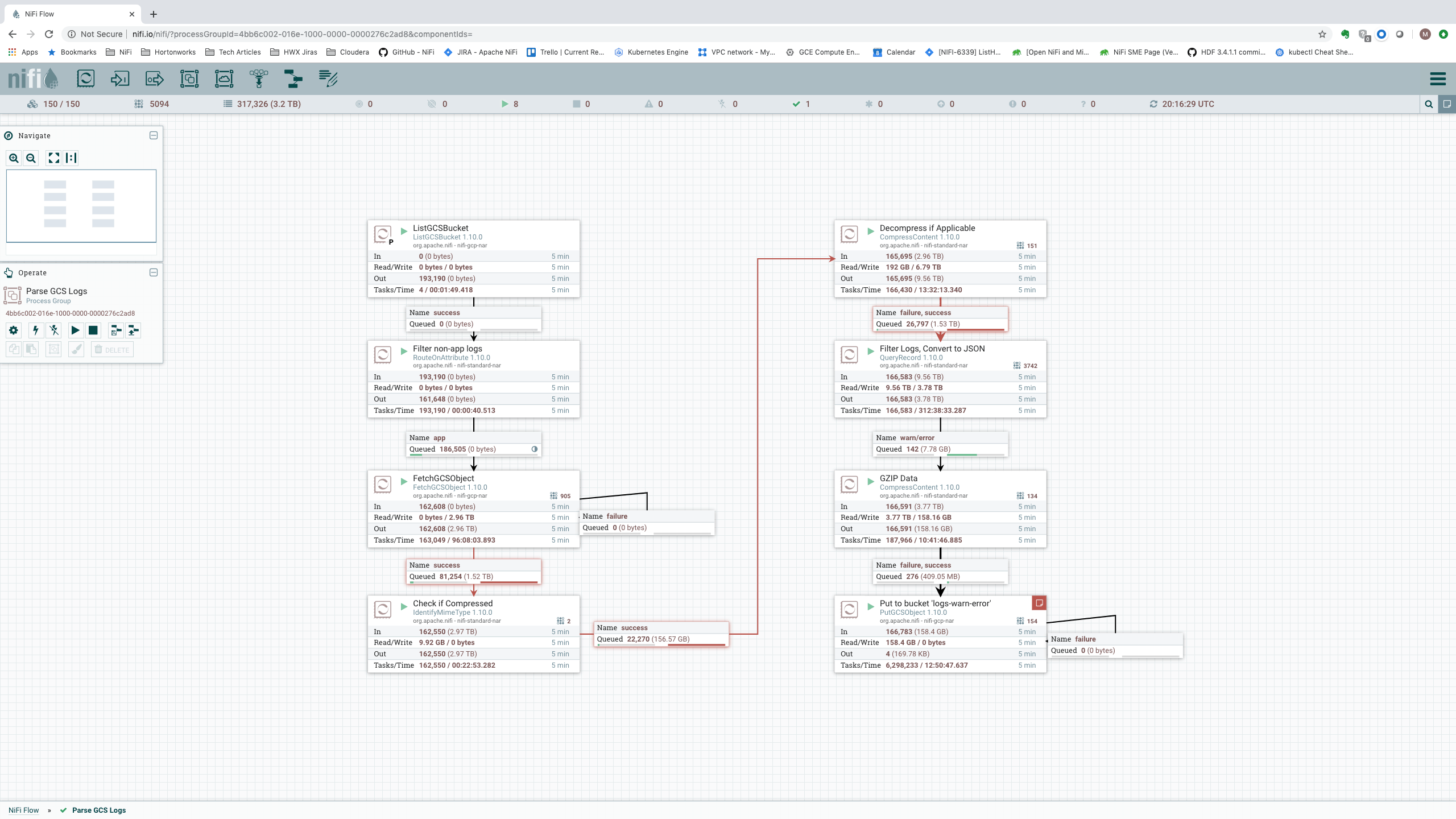
The screenshot below illustrates such a use case. Each of the Processors is denoted with a number: 1 through 8. A walk-through of the use case, which follows, references these Processor numbers in order to describe how each step is accomplished in the dataflow.

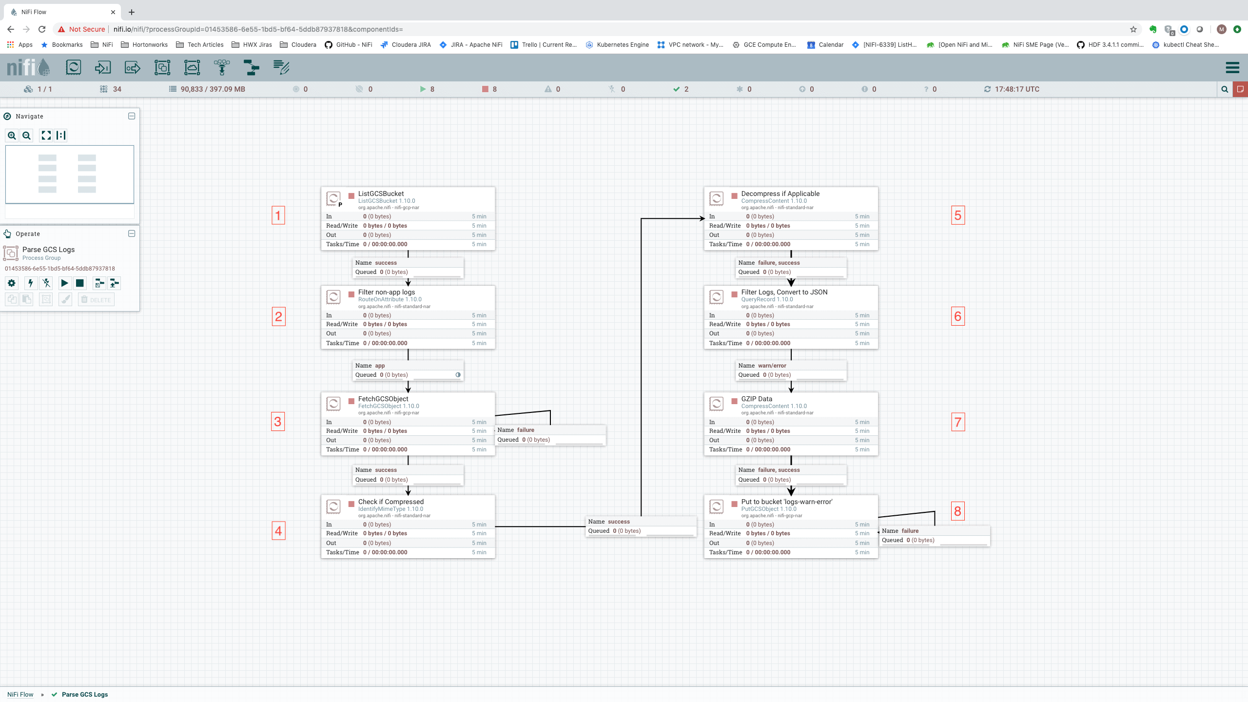
The use case that we present here is as follows:

1. There exists a Bucket in Google Compute Storage (GCS). This bucket contains about 1.5 TB worth of NiFi log data, in addition to other, unrelated data that should be ignored.
2. NiFi is to monitor this bucket [Processor 1]. When data lands in the bucket, NiFi is to pull the data if its filename contains “nifi-app”. [Processors 2, 3]
3. The data may or may not be compressed. This must be detected for each incoming log file [Processor 4]. If it is compressed, it must be decompressed [Processor 5].
4. Filter out any log messages except those that have a log level of “WARN” or “ERROR” [Processor 6]. If any Exception was included in the log message, that exception must also be retained. Also note that some log messages may be multi-line log messages.
5. Convert the log messages into JSON [Processor 6].
6. Compress the JSON (regardless of whether or not the original incoming data was compressed) [Processor 7].
7. Finally, deliver the WARN and ERROR level log messages (in compressed JSON format), along with any stack traces, to a second GCS Bucket [Processor 8]. If there is any failure to push the data to GCS, the data is to be retried until it completes.

This is a very common use case for NiFi. Monitor for new data, retrieve it when available, make routing decisions on it, filter the data, transform it, and finally push the data to its final destinations.

Note the icon on the connection between the RouteOnAttribute Processor [Processor 2] and FetchGCSObject [Processor 3]. This icon indicates that data is being load-balanced across the cluster. Because GCS Buckets do not offer a queuing mechanism, it’s up to NiFi to make pulling the data cluster-friendly. We do this by performing the listing on a single node only (the Primary Node). We then distribute that listing across the cluster, and allow all nodes in the cluster to pull from GCS concurrently. This gives us tremendous throughput and avoids having to shuffle the data around between nodes in the cluster.

Note also that we want to ensure that the data contains a good mix of WARN and ERROR messages and not just INFO level messages, because most dataflows do not filter out the vast majority of their data at the start. To this end, we caused the NiFi instances that were generating the logs to constantly error by intentionally misconfiguring some of the Processors. This resulted in about 20-30% of the log messages being warnings or errors and containing stack traces. The average message size is about 250 bytes.

Hardware

Before discussing any sort of data rates, it is important to discuss the type of hardware that is being used. For our purposes, we are using Google Kubernetes Engine (GKE) with the “n1-highcpu-32” instance type. This provides 32 cores and 28.8 GB of RAM per node (though we could get by with much less RAM, since we only use a 2 GB heap for the NiFi JVM). We will limit NiFi’s container to 26 cores to ensure that any other services that are running within the VM, such as the DNS service and nginx, have sufficient resources to perform their responsibilities.

Because NiFi stores the data on disk, we also need to consider the types of volumes that we have. When running in Kubernetes, it is important to ensure that if a node is lost, its data is not lost even if the node is moved to a different host. As a result, we store the data on Persistent SSD volumes. GKE provides better throughput for larger volumes, up to a point. So, we use a single 1 TB volume for the Content Repository in order to ensure the best performance (400 MB/sec for writes, 1,200 MB/sec for reads). We use 130 GB for the FlowFile Repository and the Provenance Repository because we don’t need to store much data and these repositories don’t need to be as fast as the Content Repository. These volumes provide built-in redundancy across the same availability zone, which gives us good performance and reliability at a good price point (currently $0.17/GB per month).

Performance

The amount of data that NiFi can process in a given time period depends heavily on the hardware but also on the dataflow that is configured. For this flow, we decided to run with a few different sized clusters to determine what sort of data rate would be achieved. The results are displayed below.

In order to really understand the data rate, and compare the rates between different cluster sizes, we should consider at which point in the flow we want to observe the statistics and which statistics are most relevant. We could look at the very end of the flow, to see how much data flowed through, but this is not a good representation because of all of the data that was already filtered out (ultimately everything but WARN and ERROR messages). We could look near the beginning of the flow, where we fetch the data from GCS, but this is also not a great representation because some of the data is compressed and some is not, so it’s hard to understand just how much data is being processed.

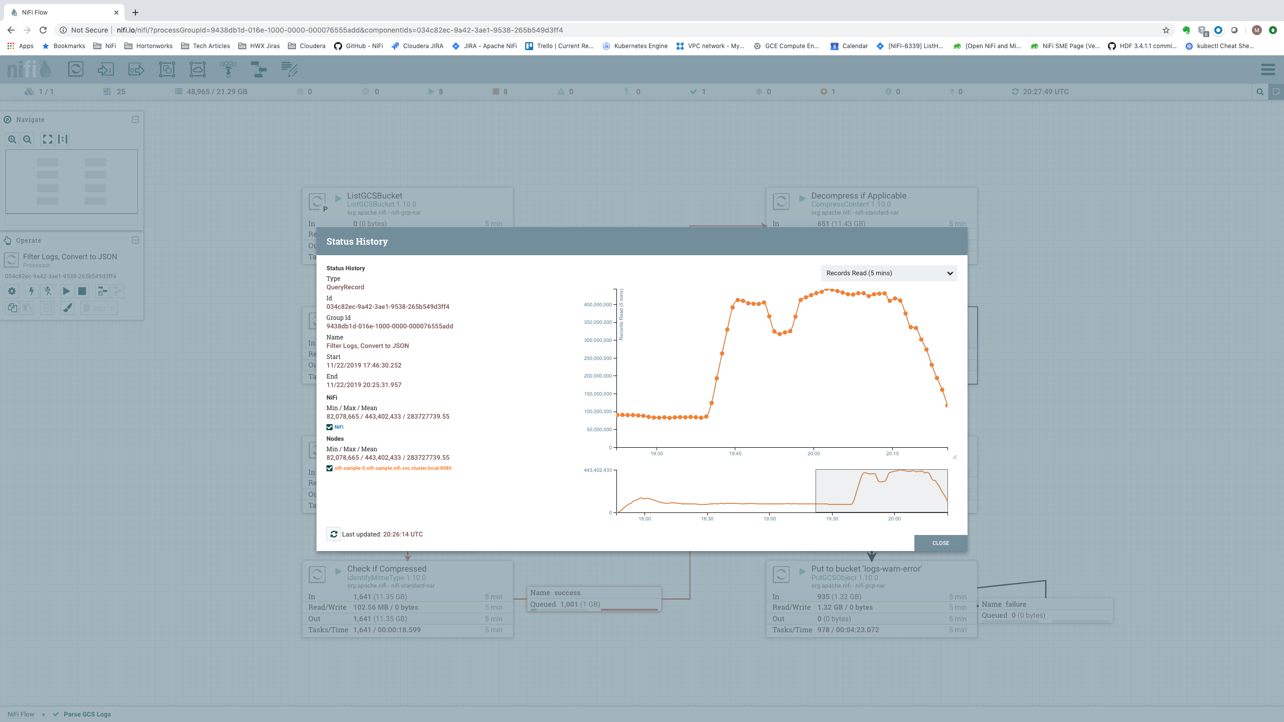
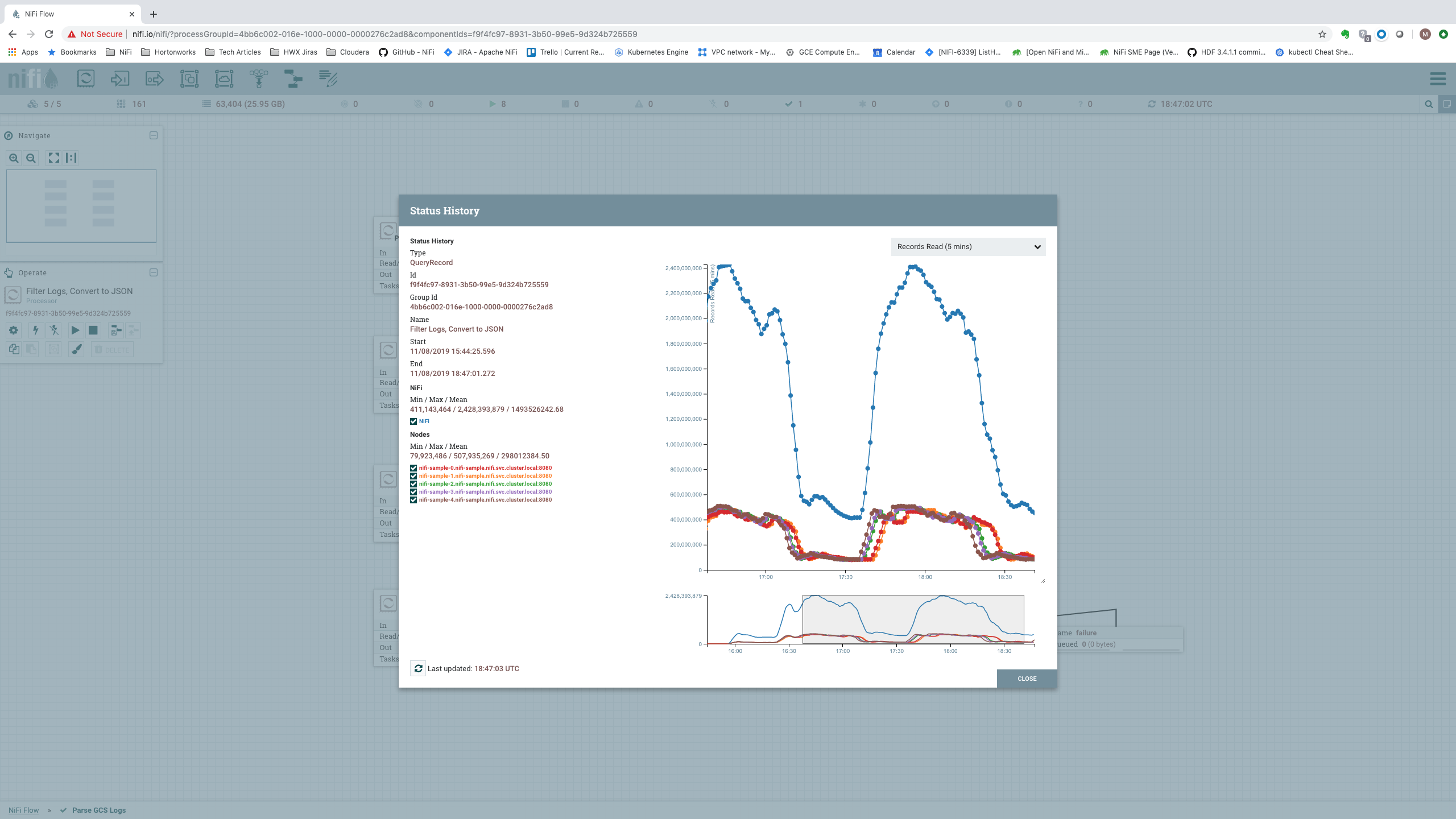
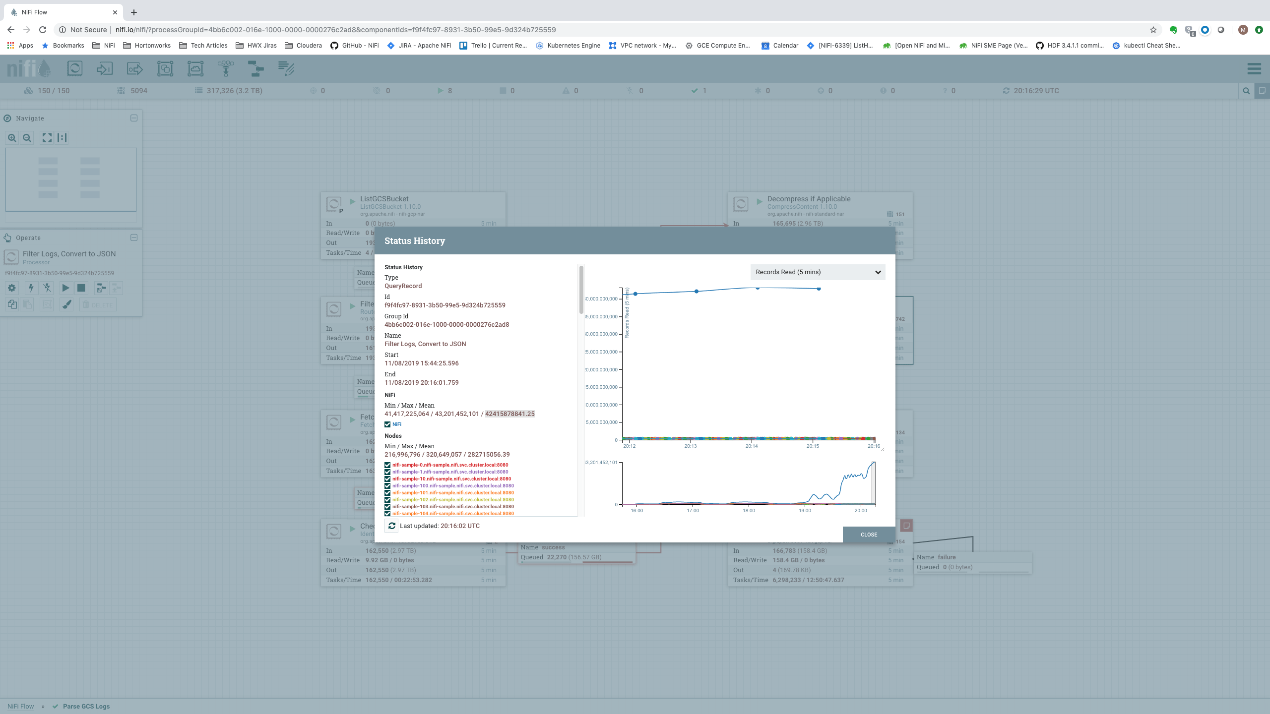
A more useful spot to consider is the input to the “Filter Logs, Convert to JSON” Processor [Processor 6]. The amount of data processed by this Processor tells us the total amount of data that the cluster was able to process. Additionally, we can look at the Status History for this Processor. This will provide us with the number of Records per second that we are processing. Both of these metrics are important, so we will consider both of them when analyzing the data rates.

Looking at these metrics, we can see how NiFi performs on this dataflow given a few different sized clusters. First, we will look at a single node:

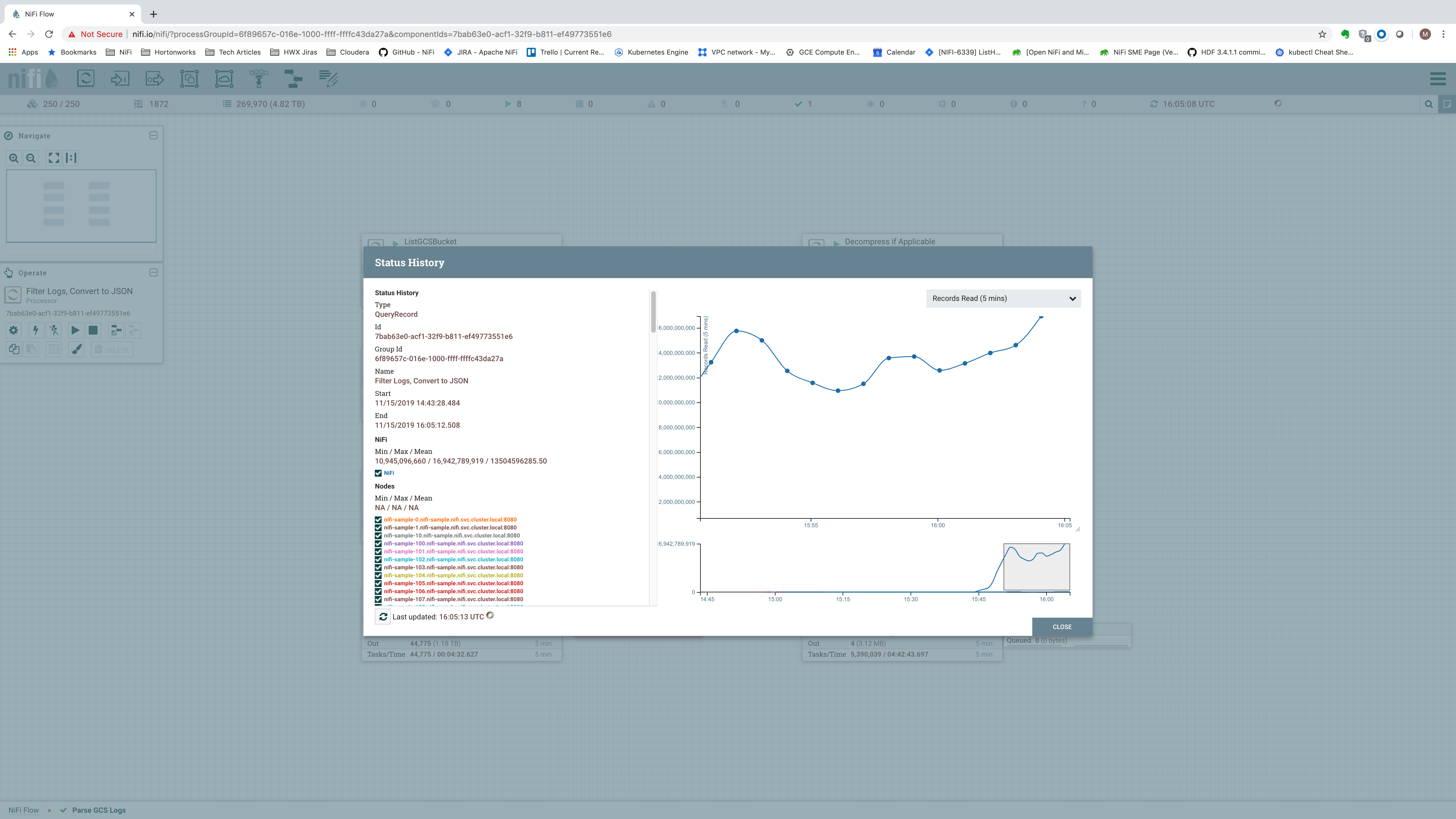
Here, we can see that the single node processed 56.41 GB of incoming data. This is over a 5 minute time window. If we divide that number by 300 seconds, we get 0.18803 GB/second, or about about 192.5 MB/sec. Looking at the Status History, we can get a feel for the number of Records (log messages) per second:

Here, we see that on average the single node processed 283,727,739 records per 5 minutes, or a little over 946,000 records per second. This is just shy of a million events per second – not shabby for a single node!

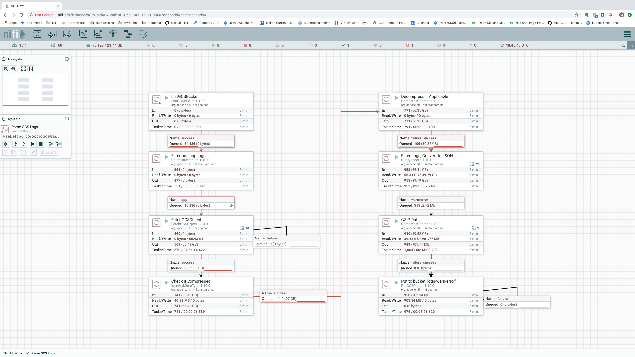
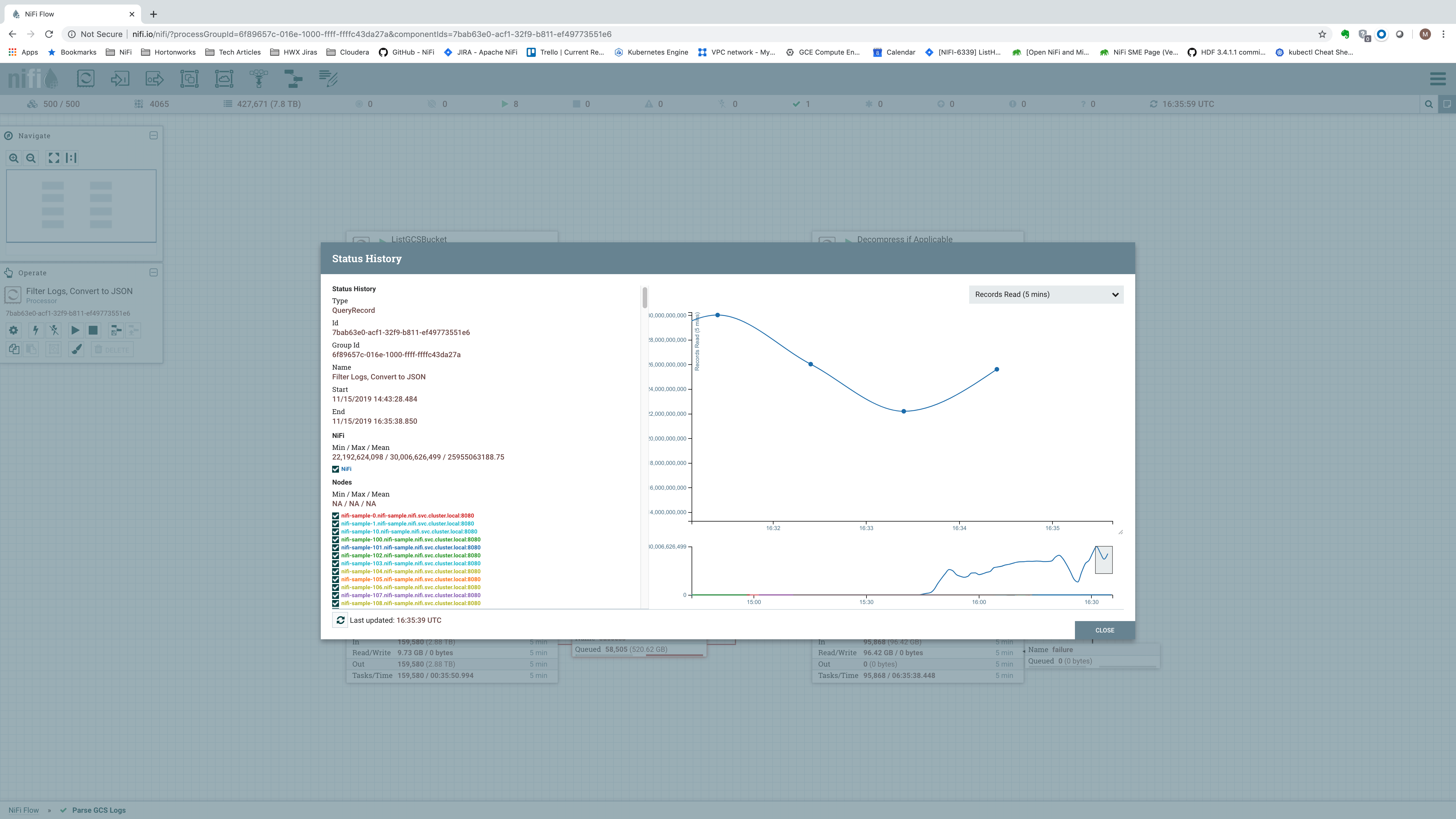
But what if a single node is not enough and we need to scale out to more nodes? Ideally, we would see that adding more nodes allows us to scale linearly. If we use a 5-node cluster instead of just a single-node cluster, we get stats that look like this:

Incoming data rate is now at 264.42 GB per five minutes (0.8814 GB/sec). In terms of records per second, we see an average of about 1.493 billion records per five minutes, or about 4.97 million records per second:

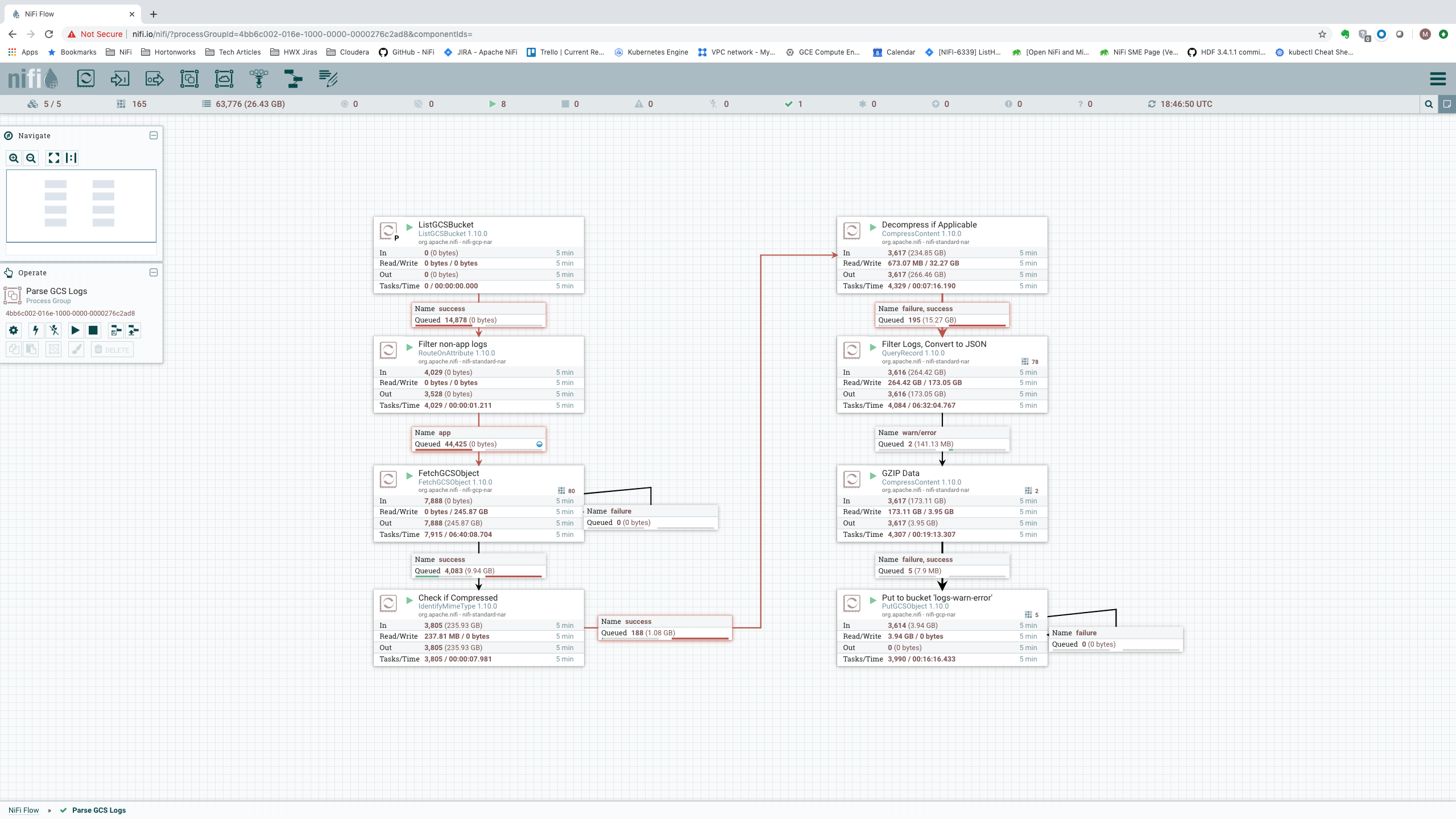
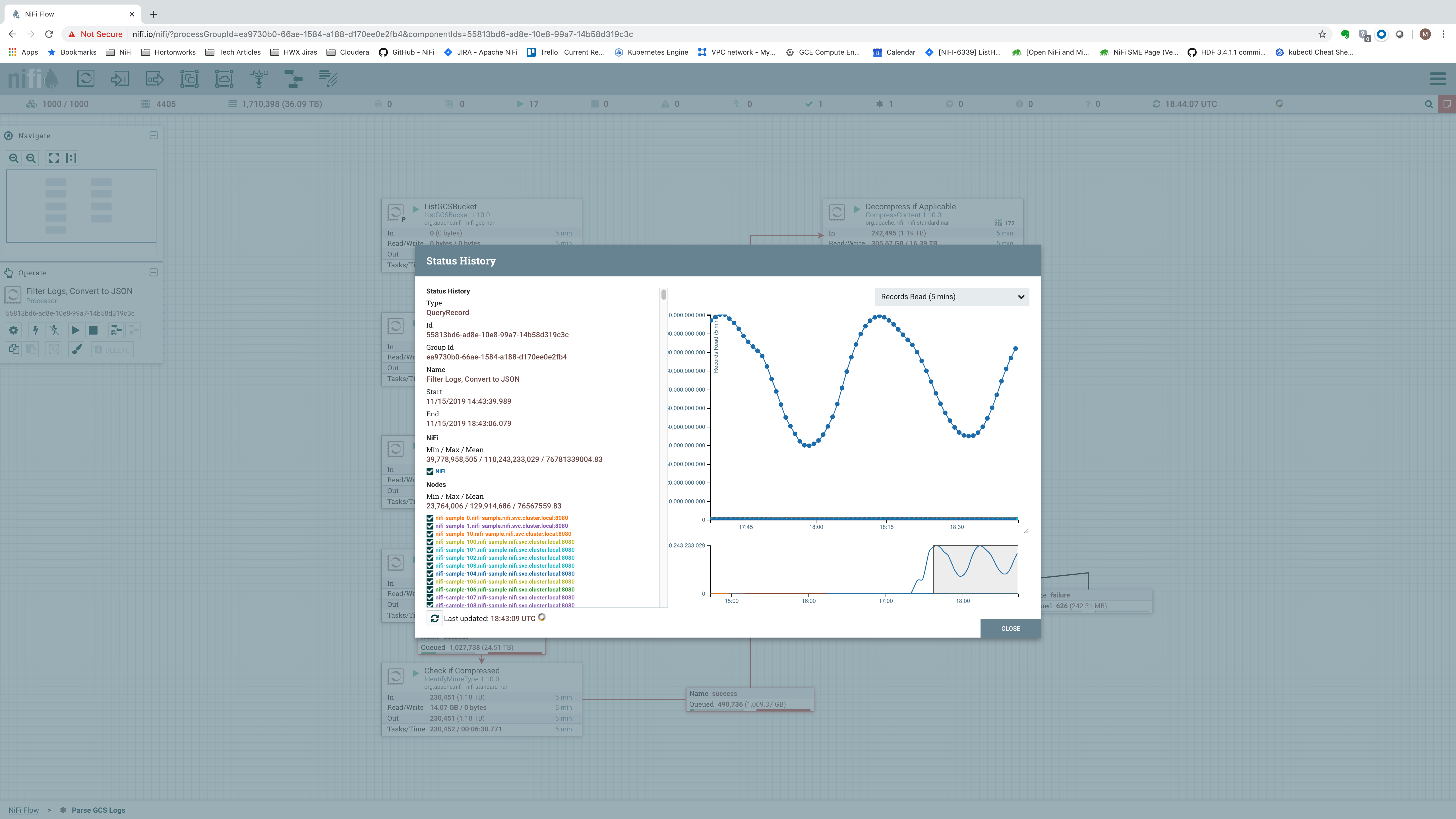
Scaling this out further, we can observe the performance achievable with a 25-node cluster:

We see an incoming data rate of a whopping 1.71 TB per 5 minutes, or 5.8 GB/sec. In terms of records per second, we show:

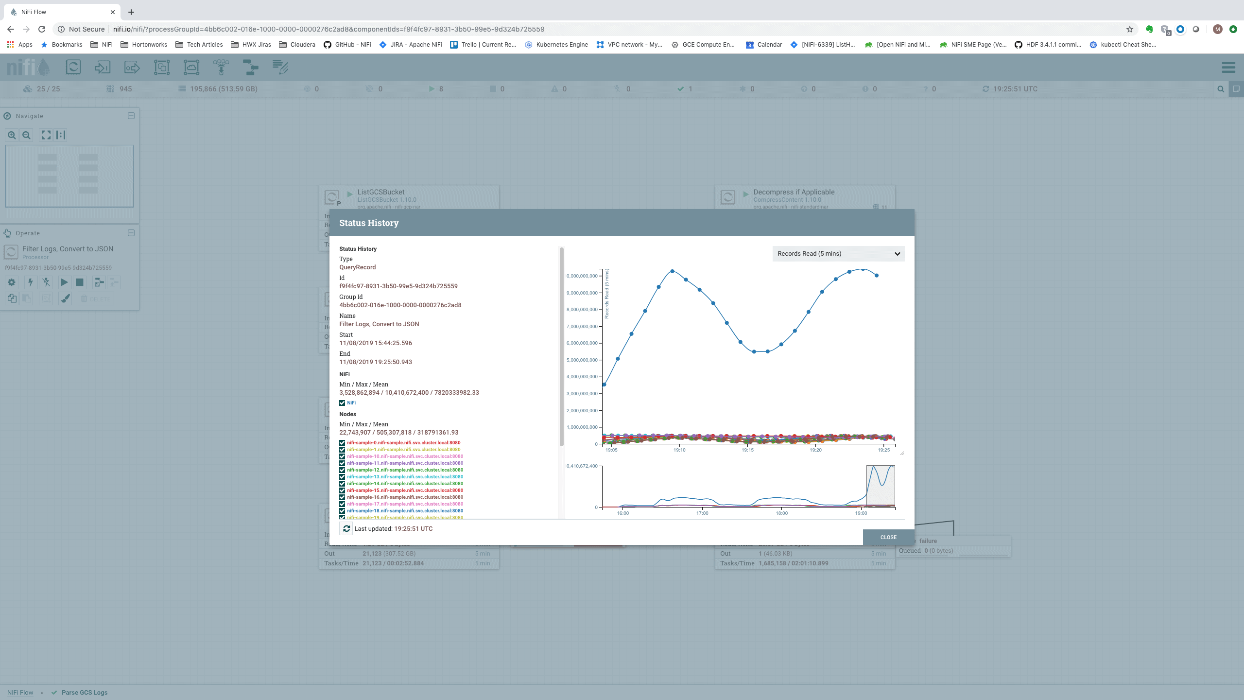
That’s a data rate of over 7.82 billion records per five minutes, or just north of 26 million events per second (or 2.25 trillion events per day). For a 25-node cluster, this equates to slightly over 1 million records/second per node.

The astute reader may note the stark variation in the number of Records Read over time as we look at the Status History. This is best explained by the variation in the data. When processing files that contain very few errors, we see a huge number of records per second. When processing messages that contain stack traces (which are much larger and require more processing), we see a lower number of records per second. This is also evidenced by comparing these stats to those of the Records Written stats:

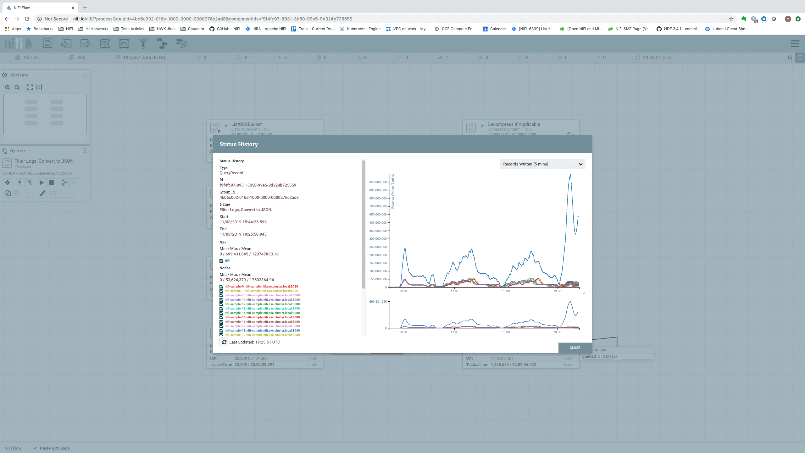
Here, we see that as the number of Records Read decreases, the number of Records Written increases and vice versa. For this reason, we make sure that when we observe the statistics, we only consider time periods that include processing both small messages and large messages. To achieve this, we select time windows where the number of Records Read reaches a high point as well as a low point. We then consider the average number of Records Read over this time period.

At 26 million events per second, most organizations have easily reached their necessary data rates. For those who haven’t, though, will NiFi continue to scale linearly as we reach larger clusters?

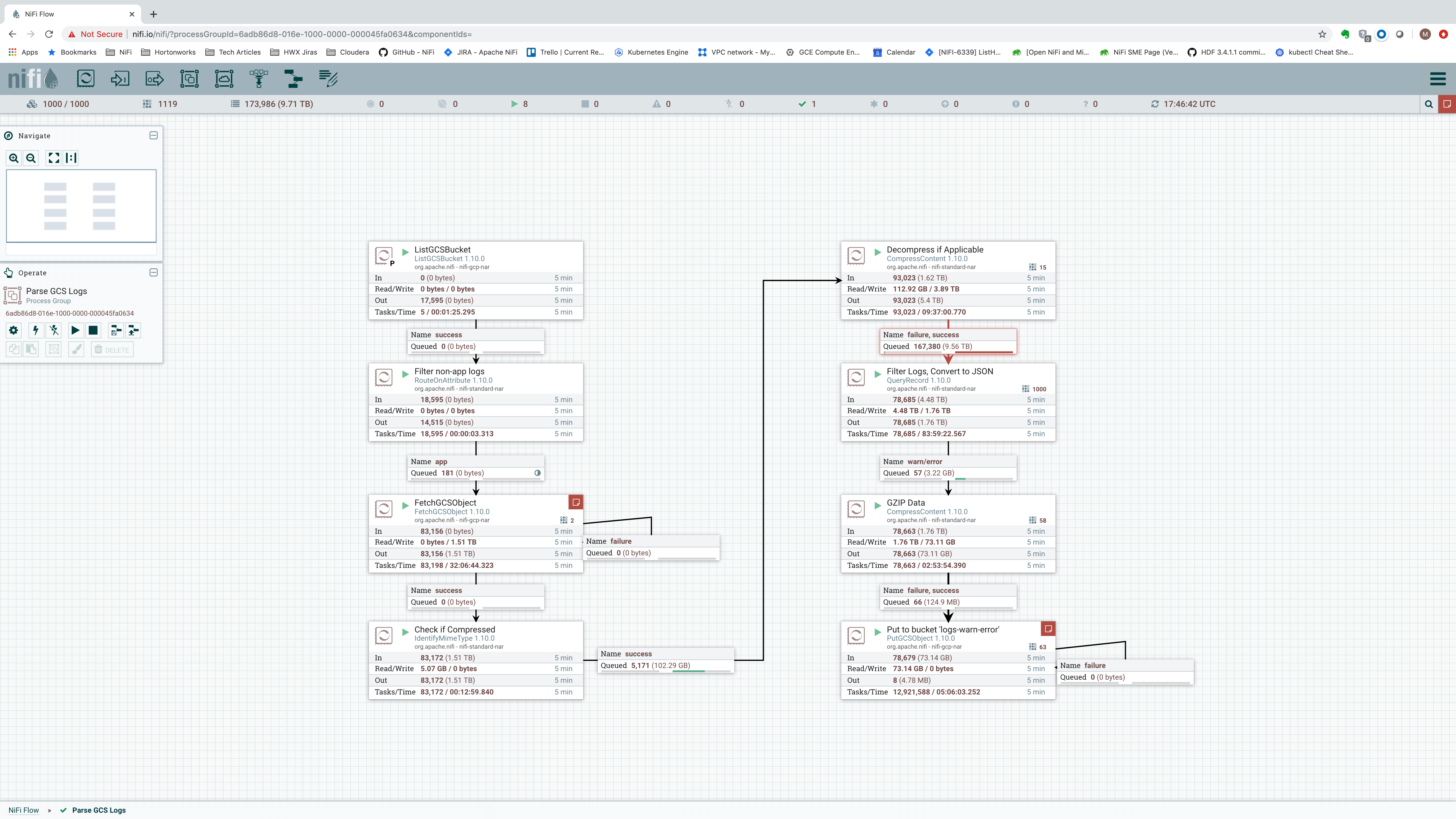
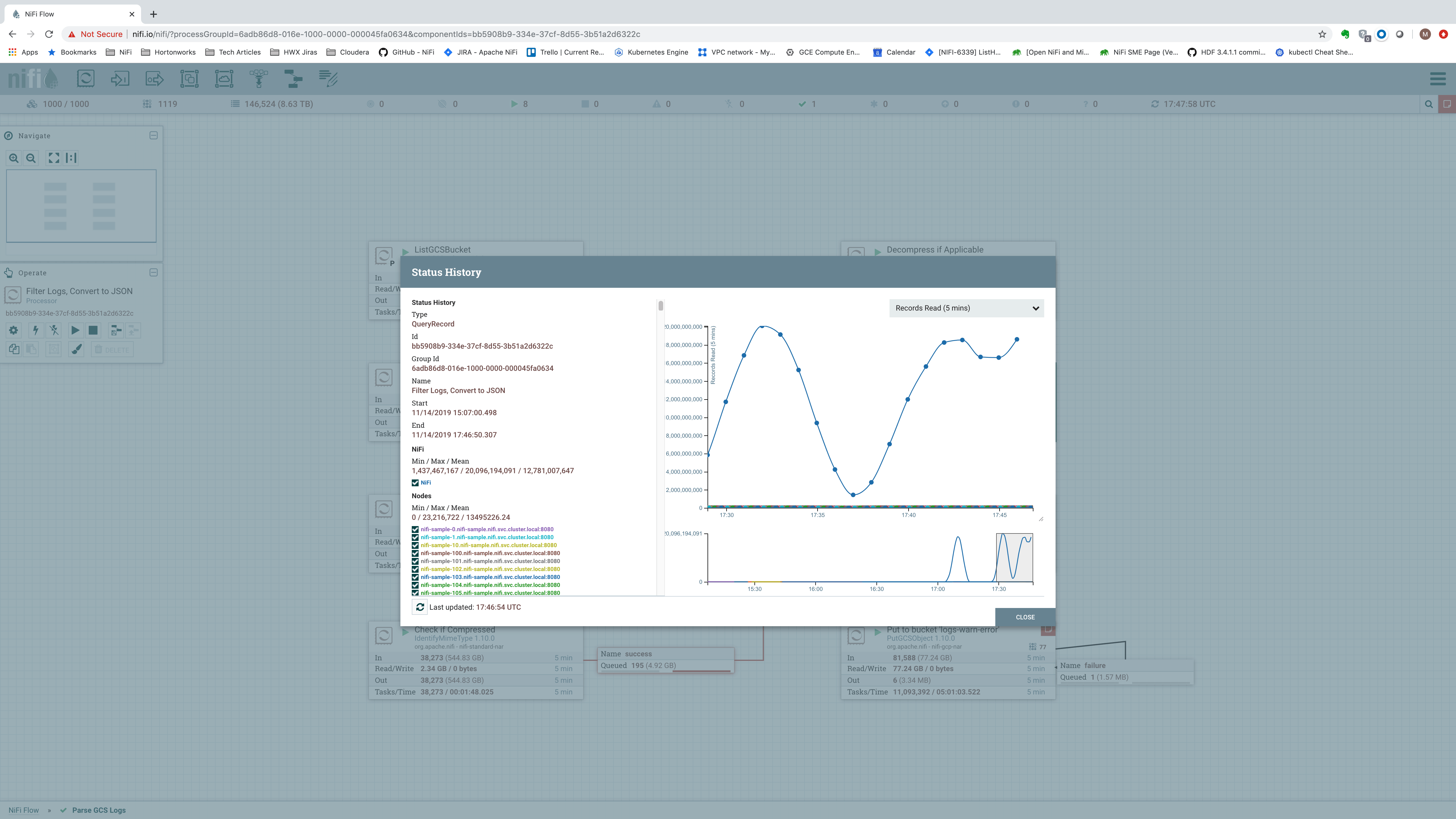
To find out, we increased the cluster from 25 nodes to 100 nodes and then to 150 nodes. The results obtained for the 150-node cluster are shown here:

Here, NiFi handles the data at an impressive rate of 9.56 TB (42.4 billion messages) per 5 minutes, or 32.6 GB/sec (141.3 million events per second). That equates to 2.75 PB (12.2 trillion events) per day! All with granular provenance information that tracks and displays every event that occurs to the data. When and where the data was received; how it was transformed; and when, where, and exactly what was sent elsewhere.

The table below summarizes the data rates achieved, for comparison purposes:

Nodes	Data rate/sec	Events/sec	Data rate/day	Events/day
1	192.5 MB	946,000	16.6 TB	81.7 Billion
5	881 MB	4.97 Million	76 TB	429.4 Billion
25	5.8 GB	26 Million	501 TB	2.25 Trillion
100	22 GB	90 Million	1.9 PB	7.8 Trillion
150	32.6 GB	141.3 Million	2.75 PB	12.2 Trillion

Data rates and event rates captured running the flow described above on Google Kubernetes Engine. Each node has 32 cores, 15 GB RAM, and a 2 GB heap. Content Repository is a 1 TB Persistent SSD (400 MB/sec write, 1200 MB/sec read).

Scalability

While it’s important to understand the performance characteristics of your system, there exists a point at which the data rate is too high for a single node to keep up. As a result, we need to scale out to multiple nodes. This means that it is also important to understand how well a system is able to scale out.

We saw in the previous section that NiFi can handle scaling linearly out to at least 150 nodes, but where is the limit? Can it scale to 250 nodes? 500? 1000? What if these nodes are much smaller than the afore-mentioned 32-core machines? Here, we set out to find the answers.

In order to explore how well NiFi is able to scale, we tried creating large clusters with different-sized Virtual Machines. In all cases, we used a VM that has 15 GB of RAM. We also used much smaller disks than in the previous trials, using a 130 GB volume for the Content Repository, a 10 GB volume for the FlowFile Repository, and a 20 GB volume for the Provenance Repository. These smaller disks mean much lower I/O throughput because the number of IOPS and MB/sec are limited with smaller disk sizes. As such, we would expect a cluster with the same number of nodes to yield a much smaller throughput than in the previous section.

4-Core Virtual Machines

We first tried scaling out to see how NiFi would perform using very small VM’s, with only 4 cores each. Because each VM must host not only NiFi but also a Kubernetes DNS service and other Kubernetes core services, we had to limit the NiFi container to only 2.5 cores.

A cluster of 150 nodes worked reasonably well, but the UI demonstrated significant lag. Scaling to 500 nodes meant that the user experience was severely degraded, with most web requests taking at least 5 seconds to complete. Attempting to scale to 750 nodes resulted in cluster instability, as nodes began to drop out of the cluster. NiFi’s System Diagnostics page showed that the Cluster Coordinator had a 1-minute Load Average of more than 30, with only 2.5 cores available. This means that the CPU was being asked to handle about 12 times more than it was able to handle. This configuration – 4 cores per VM – was deemed insufficient for a 750-node cluster.

6-Core Virtual Machines

Next, we tried to scale out a cluster of 6-core Virtual Machines. This time we were able to limit the container at 4.5 cores instead of 2.5 cores. This provided significantly better results. A 500-node cluster did demonstrate some sluggishness but most web requests completed in less than 3 seconds.

Scaling out to 750 nodes made little difference in terms of UI responsiveness. Next, we wanted to try a cluster of 1,000 nodes.

We were, in fact, able to scale out to 1,000 nodes this time, using 6-core VM’s! The cluster remained stable, but of course, with these small VM’s and limited disk space, the performance was certainly not in the range of 1 million events per second on each node. Rather, the performance was in the range of 40,000-50,000 events per second on each node:

In this setup, the UI was still a bit sluggish, with most requests taking in the range of 2-3 seconds.

Because we have such few cores, we also decreased the number of threads that we provided NiFi for running the flow. We can see that the nodes were not utilized too heavily, with the one-minute load average generally ranging from 2 to 4 on a 6-core VM:

The question remained, though, if scaling out to this degree still results in linear scale. We examined this next.

12-Core Virtual Machines

We conclude our exploration of NiFi’s scalability by scaling out to 1,000 nodes using 12-core Virtual Machines. We gathered performance metrics with 250 nodes, 500 nodes, and 1,000 nodes in order to determine if the performance scaled linearly. Again, these nodes contained only about one-third the number of cores as in the previous example and had much slower disks, so the performance here should not be comparable to the performance of the larger VM’s.

With 250 nodes, we saw the number of events processed at about 45 million events/sec (180,000 events/second per node) with these VM’s:

With 500 nodes, we saw the number of events processed at around 90 million events/sec (180,000 events/second per node) again:

This is about 20% of the performance that we saw from the 32-core systems. This is very reasonable, considering that the node has 1/3 the number of cores and the Content Repository provides about 1/4 the throughput of those in the 32-core system. This indicates that NiFi does in fact scale quite linearly when scaling vertically, as well.

Finally, we scaled the cluster of 12-core VM’s to 1,000 nodes. Interestingly, this posed a slight problem for us. With a 1,000-node cluster, the 1.5 TB of log data was processed so quickly that we had trouble keeping the queues full for a long enough period of time to get an accurate performance measurement. To work around this, we added a DuplicateFlowFile processor to the flow, which would be responsible for creating 25 copies of each log file that is fetched from GCS. This would ensure that we don’t run out of data so quickly.

This, however, is a bit of a cheat. It means that for 96% of the data, we aren’t fetching it from GCS because the data already resides locally. However, NiFi did still process all of the data. As a result, we would expect to see the performance numbers a bit higher than double those of the 500-node cluster.

And sure enough, we ended up with results on the order of 256 million events per second for the cluster, or 256,000 events/second per node.

Bringing It All Together

With NiFi, our philosophy has always been that it’s not just about how fast you can move data from Point A to Point B; it’s about how fast you can change your behavior in order to seize new opportunities. This is why we strive to provide such a rich user experience to build these dataflows. In fact, this dataflow only took about 15 minutes to build and can be changed on the fly at any time. But with numbers that eclipse 1 million records per second on each node, it’s hard not to get excited!

Couple that with the fact that NiFi is capable of scaling out linearly to at least 1,000 nodes and that vertical scaling is linear as well. Multiply 1 million events per second by 1,000 nodes. Then consider that we can likely scale out further, and that we can certainly scale up to 96 cores per VM. This means a single NiFi cluster can run this dataflow at a rate well over 1 billion events per second!

When architecting any technical solution, we need to ensure that all tools are capable of handling the volume of data anticipated. While any complex solution will involve additional tools, this article demonstrates that NiFi is unlikely to be the bottleneck when properly sized and running a well designed flow. But if your data rate does exceed a billion events per second, we should talk!