


It’s been over two years now that Google launched Smart Reply, a feature for Gmail that automatically suggests short replies for users’ emails. Behind this technology are many natural language processing (NLP) models that allow this program to process and understand human language.
We have seen in a previous post that methods such as GloVe or FastText can be used to produce word embeddings. More interestingly, these embeddings are the building blocks of sentence representations which are key to building programs such as Google’s Smart Reply.
Most successful approaches for computing these representations involve training a deep learning model. For instance, we will go over InferSent, a model that uses recurrent neural networks to produce sentence embeddings. But the question is: how deep does a sentence embedding model need to be?
There is a common misconception that deep learning is required for achieving good sentence representations, as actually simple methods can be just as effective. Specifically, we will go over SIF embeddings, a statistical method that computes sentence embeddings using a simple word vector averaging.
How to Evaluate Sentence Embeddings?
It seems that they are as many ways of evaluating sentence embeddings as there are NLP tasks where these embeddings are used. As a result, there isn’t a single universal notion of what a good sentence representation is.
One way sentence embeddings are evaluated is using the Semantic Textual Similarity (STS) task. The idea of STS is that a good sentence representation should encode the semantic information of a sentence in order to be able to differentiate between similar sentences and dissimilar ones. In practice, we evaluate the ability of a model to recognize similar sentences by computing the cosine similarity of many couples of sentences, each labeled with a similarity score between 0 and 5, then looking at how these scores correlate with computed cosine similarities.
The interesting thing about STS is that we don’t use anything else but the raw sentence embeddings themselves. In particular, this allows to evaluate an embedding technique without introducing the specificities of a model trained for a specific task.
Sparse Representations and BOW
Probably one of the most straightforward sentence embedding techniques is Bag Of Words (BOW). This method assumes that two sentences are similar if both sentences use the same words. Therefore, the sentence representation is simply a vector of word counts, which can also be seen as a sum of one-hot vectors.
Note: The values in a BOW representation are not always word counts. Sometimes, these are replaced with the more robust TF-IDF weights.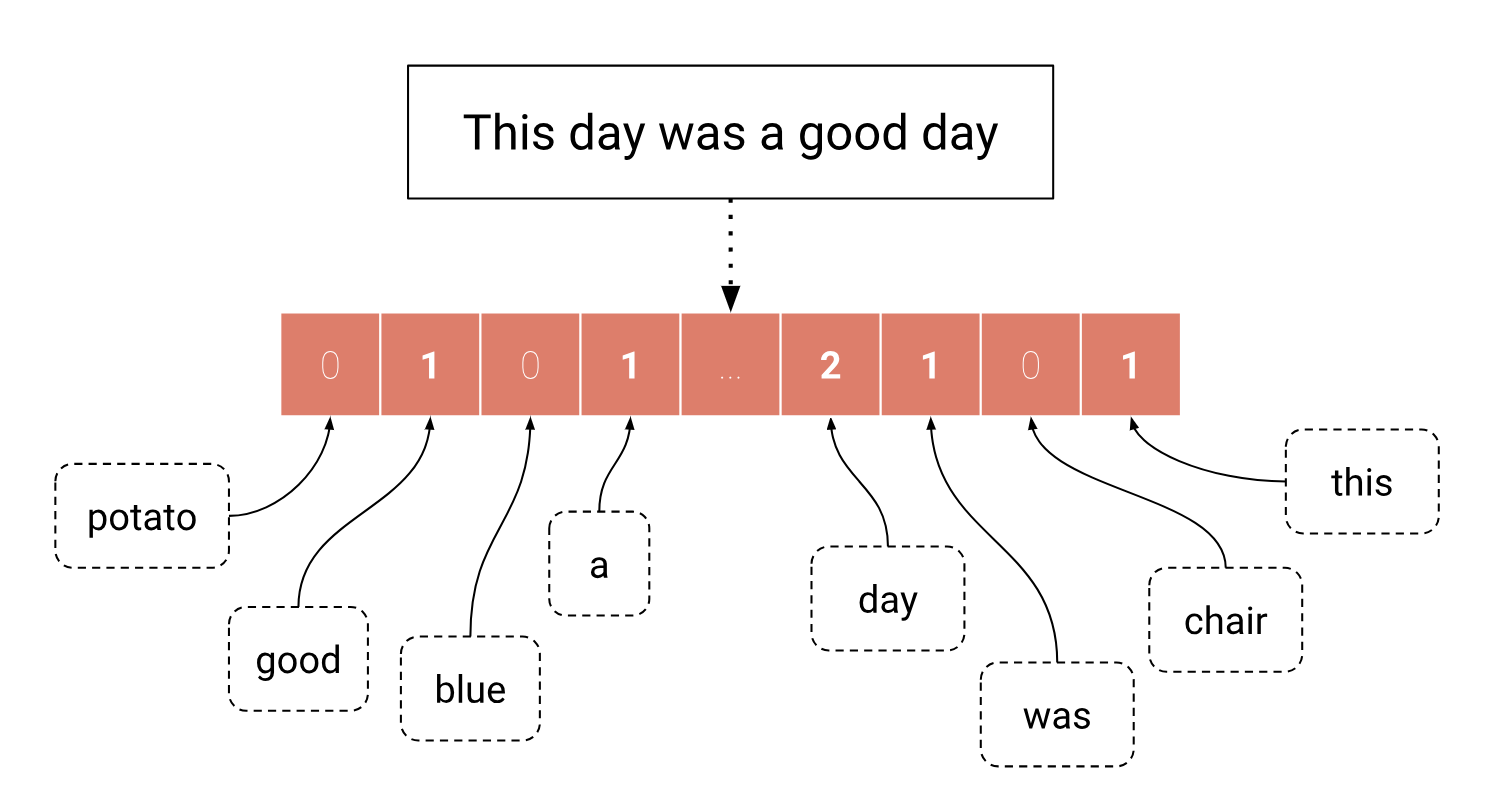
While simple, these representations are not ideal. In fact, since the vectors get longer with the number of different words in the training data, BOW vectors are usually very large. Moreover, only a small portion of these words ever occur in any given sentence, thus making the representation sparse. Another issue with these representations is that we can’t really use them for computing the similarity between sentences. In fact, computing the cosine similarity of two sentences that use different words (for example: “A dark-colored phone” and “This black smartphone”) would systematically yield a score of zero, despite the sentences being similar or not.
In spite of its many downsides, Bag-of-Words is usually a good baseline for text classification, especially for small datasets and when combined with linear models that can handle sparsity. But when it comes to more complex NLP tasks such as Machine Translation or Named Entity Recognition, BOW is quickly cast aside for more expressive dense representations.
2. InferSent, a Dense Representation
Neural Networks were successfully used in Computer Vision, first pre-trained on large datasets such as ImageNet, then used on various downstream tasks. This transfer learning is achieved by re-using the previous “understanding” of images from the original dataset onto new images. Naturally, we can wonder if it is possible to achieve a similar thing in NLP with texts.
In 2017, Conneau et al. [paper][code] proposed using the Stanford Natural Language Inference (SNLI) dataset for NLP in the same way ImageNet was used for Computer Vision. SNLI is a dataset for Textual Entailment, which is the task of classifying couples of sentences as either entailment (i.e. logical implication), contradiction, or neutral (neither of the previous classes).
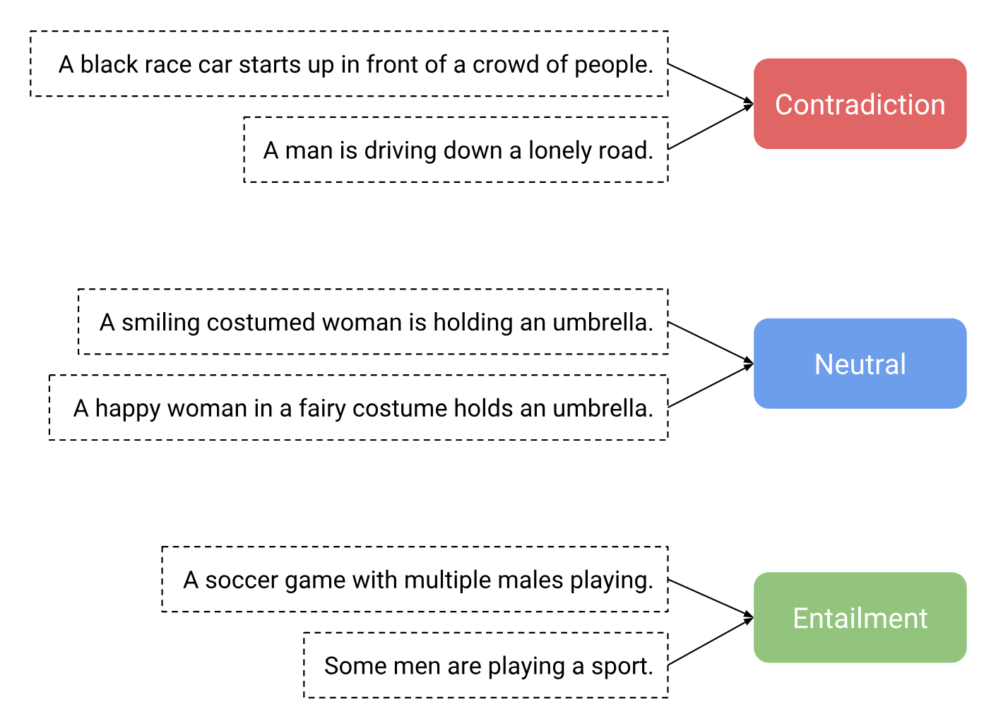
The authors’ idea is that by training a deep learning model to be able to perform a Textual Entailment task, we would learn a way of encoding sentences into meaningful numerical representations that can be used in other NLP tasks.
There are many ways a sentence can be encoded. In fact, the authors tested different architectures such as Hierarchical ConvNets and LSTMs with self-attention, but the best encoder — both on the SNLI pre-training task and on the tested transfer tasks — was the following bi-LSTM with max-pooling.

This encoder feeds pre-trained GloVe embeddings to a bi-LSTM that processes a sequence of words in both regular and reverse order. The output word representations are then max-pooled over the “time dimension”. On the diagram above, this means that the maximum is computed over the horizontal axis (this is why the arrows are crossing), producing the final sentence embedding.
Note: Using a bi-LSTM instead of a plain LSTM allows for more expressivity by using more context. Bi-LSTMs are a way of judging the “usefulness” of a word using both the previous and the next words in the sentence.
This model is called InferSent and it works pretty well in practice. In fact, when the model came out, it outperformed most previous models on a large number of transfer tasks from binary and multi-class classification to STS.
But do we really need such a complex model to learn good sentence representations ? Can’t we just average the individual word embeddings to get meaningful embeddings for entire texts ? Well actually, we can.
Simpler Yet Effective Sentence Representations
Deep Averaging Network (2015)
In 2015, Iyyer et al. showed that a strong baseline for text classification could be achieved using Deep Averaging Networks (DAN). These DANs consists in averaging all the word embeddings of a sentence before feeding this representation to multiple feed forward layers. In their paper, the authors showed that DANs achieved comparable results to the more complex Recursive Neural Networks on tasks like sentiment analysis and question answering while being a lot simpler (and faster).
A year later, Wieting et al. did a more extensive benchmark including among others: DANs, LSTMs and a plain average of word embeddings. They observed that the plain averaging could achieve similar performance to LSTMs and even sometimes outperform these on tasks like textual similarity.
SIF embeddings (2016)
One year later, Arora et al. [paper][code] developed a simple sentence embedding technique called SIF embeddings (Smooth Inverse Frequency), that computes sentence embeddings as a weighted average of word vectors. This model is backed by some interesting theory that is worth a quick review.
To build this model, the authors make the following assumptions:
- The generation of a corpus can be seen as a dynamic process where the
t-th word is produced at stept. This process is driven by a vectorc(t)called the discourse vector, which models “what is being talked about”. - To a word
w, we denote its vector representation byv(w). - The probability that a word
wis emitted at timetis proportional to the similarity between the word and the discourse at timet:

The authors also assume that the discourse vector c(t) does a slow random walk. This basically means that for any given sentence s, the discourse vector doesn’t change much and so can be considered constant. This sentence discourse vector c(s) models “what is being talked about in the sentence” and is the sentence embedding we are looking for.
Under the previous assumptions, the authors show that the sentence discourse vector is estimated using Maximum A Posteriori (MAP) as the average of the individual word vectors. [Arora et al. 2016, theorem 1]
But this model is too simplistic and doesn’t handle the fact that out of context words may occur regardless of the discourse. Moreover, the authors observed that there was a common component in the sentence representations computed by averaging word vectors. The most similar words to that component are found to be syntax-related: “just” “up” “but” “while”… This motivated them to adapt the model by introducing two new parameters α and β along with a discourse vector, common to all sentences, denoted by c(0) :

Let’s go over this new model:
- If both α and β are 0, we fall back on the previous model.
- If α>0, any word can appear in s thanks to its sheer frequency
p(w). - If β>0, words that are correlated with
c(0)can appear.
Using Maximum Likelihood Estimation, the authors show that:

where a is a smoothing hyper-parameter that depends on α and Z.
But this is still not the sentence embedding we are after. In fact, if we recall the formula:

we see that we still need to remove the common discourse vector c(0).
Since c(0) and c(s) are orthogonal, and since c(0) is common to all the representations obtained as a weighted average of word vectors, the authors propose removing the first component of these representations using SVD.
c(0).
In short, SIF embeddings can be computed this way:
- First, compute all the frequencies of all the words of your corpus.
- Then, given a hyper-parameter
ausually set to1e-3,and a set of pre-trained word embeddings, compute the weighted average above for each of your texts/sentences. - Finally, Use SVD to remove the first component off of these averages and get fresh sentence embeddings.
Considering their simplicity, SIF embeddings perform very well. In fact, this method can even outperform state-of-the-art deep learning techniques such as InferSent on semantic textual similarity tasks. This is interesting because SIF doesn’t care about word order at all while InferSent uses LSTMs which integrate this information into their representations. This could mean that SIF embeddings are much better at encoding semantic information than simple recurrent neural networks. But when it comes to classification tasks, SIF slightly lags behind its deep counterparts. This is probably because averaging word embeddings doesn’t provide a representation that is complex enough to solve tasks such as sentiment analysis.
Conclusion
All in all, both deep and non-deep models produce good sentence representations, so an important thing to keep in mind is that we don’t always need deep learning to get good sentence embeddings. As a general rule, it seems that simple techniques such as SIF are sufficient when the goal is to encode the global meaning of a sentence. This could explain why these methods often beat state-of-the-art deep learning techniques on tasks such as semantic text similarity or paraphrase detection. On the other hand, they perform less on tasks like sentiment analysis and sequence labelling where we need to detect something more specific than just the global meaning of the sentence. On these tasks, deep learning models that rely on recurrent neural networks like LSTMs (see ULMFiT) or other complex mechanisms such as attention (see the this model from OpenAI as well as BERT) seem to be more appropriate.
So as a final recommendation, we would advise to always start with a strong baseline using a simple and fast method like SIF before advancing to more complex methods.