


As many real-world problems can naturally be modeled as a network of nodes and edges, Graphical Neural Networks (GNNs) provide a powerful approach to solve them. By leveraging this inherent structure, they can learn more efficiently and solve complex problems where standard machine learning algorithms fail.
In this context, the first article of this series on GNNs discusses the benefits of such models when it comes to classifying entities in a network or predicting a continuous attribute.
But what if the task to be solved is about predicting the existence of a relationship between entities or a characteristic of this relationship?
Real-life examples are abundant:
- Retailers are interested in predicting the satisfaction score that consumers would give to their products in order to improve their recommendation tool.
- Social networks would find it useful to predict the likelihood that two users connect to improve their suggestions and ultimately help each of them expand your network.
- Chemists study the existence of interactions between molecules in order to discover new drugs or to avoid unexpected side effects when taking several drugs.
The previous article only considers homogeneous graphs, that is, graphs with a single type of node. What if the network contains different types of entities? For instance, in their modeling, retailers need to account for customers and products as different types of nodes, social networks users and content, etc. This type of graph is commonly called a heterogeneous graph.
Objective
This article focuses on building GNN models for link prediction tasks for heterogeneous graphs.
To illustrate these concepts, I rely on the use case of recommendation. More specifically, predict the rating that users will give to a movie. I also discuss the benefits of using graph-based models by comparing them to a more traditional approach, collaborative filtering.
After reading this article, you will understand:
- What is SAGEGraph and to what extent does it improve the GCN approach?
- How is link prediction performed using GNNs models?
- How can GNNs models be applied to real-world problems?
This article is the second part of three-part series that aims to provide a comprehensive overview of the most common applications of GNN models to real-world problems. While the second focuses on link prediction, the two others tackle respectively node classification and graph classification.This article assumes minimal knowledge of GNNs (you can refer to the first article of the series). The experimentations described in the article were carried out using the libraries PyTorch Geometric, Surpise, and Plotly.
You can find the code here on GitHub.
1. Link Prediction Model: What's Under the Hood?
Before getting into the use case, let’s start with some theory.
First, we introduce the GNN layer used, GraphSAGE. Then, we show how the GNN model can be extended to deal with heterogeneous graphs. Finally, we discuss possible approaches that use node embeddings for link prediction.
1.1 GraphSAGE
A first natural question is: Why shift from standard GCN to GraphSAGE?
GCNs suffer from several issues caused by their very learning framework:
- Difficulties in learning from large networks: GCNs require the presence of all the nodes during the training of the embeddings. This does not allow the model to be trained in batches.
- Difficulties to generalize to unseen nodes: GCNs assumes a single fixed graph. But, in many real-world applications, the embeddings of unseen nodes need to be quickly generated (e.g., posts on Twitter, videos on YouTube, etc.)
As a result, GCNs are not very practical, limited in terms of memory when handling large networks, and even not suitable for some cases.
GraphSAGE overcomes the previous challenges while relying on the same mathematical principles as GCNs. It provides a general inductive framework that is able to generate node embeddings for new nodes.
Introduced by the paper Inductive Representation Learning on Large Graphs [1] in 2017, GraphSAGE, which stands for Graph SAmpling and AggreGatE, has made a significant contribution to the GNN research area.
So how does GraphSAGE work concretely?
Rather than training individual embeddings for each node, the model learns a function that generates embeddings by sampling and aggregating the features of the local neighborhood of a node.
At each iteration, the model follows two different steps:
- Sample: Instead of using the entire neighborhood of a given node, the model uniformly samples a fixed-size set of neighbors.
- Aggregate: Nodes aggregate information from their local neighbors as shown in the equation below. In the original paper [1], three aggregation functions are considered:
- Mean aggregator:
It consists in taking the average of the vectors of the neighboring nodes.
Simple and efficient, this approach has led to good performances in the experiments carried out in the research paper. It is the one that has been retained in the application below.
- LSTM aggregator:
This aggregator has the potential to benefit from the greater expressive capabilities of the LTSMs architecture. To adapt it to graphs that have no natural order, the aggregator is applied to a random permutation of the node’s neighbors. - Pooling aggregator:
It consists in feeding a fully connected neural network with the vector of each neighbor. After this transformation, a maximum pooling operation per element is applied to aggregate the information on all the neighbors.
It has yielded very good results in the experiments with the paper.
These steps are repeated for all nodes K times (usually K= 2 is enough). Therefore, as these steps are repeated for all nodes, nodes gradually acquire more and more information from more distant areas of the graph. The figure below illustrates the process for K=2.
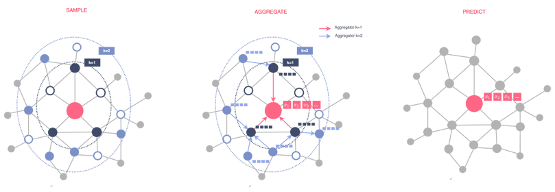
Figure 1 - Illustration of GraphSAGE approach, illustration by Lina Faik, inspired by [1]
Note that the weights used in the aggregation step are not specific to a node but only specific to iteration k. Therefore, they are shared by all the neighborhoods making generalization to unseen nodes possible.
To sum up, you can consider GraphSAGE as a GCN with subsampled neighbors.
1.2 Heterogeneous Graphs
Consider movie recommendations, as illustrated in the figure below.
Goal: Predict the rating that a given user is likely to give to the most recent movies. This prediction would then be used to suggest the most relevant movie.
Modeling: The problem can be modeled as a graph with two types of nodes: one representing users and the other movies. A user node is linked to the movie node if the user has rated the movie and is labeled with the rating.
Task: Under this modeling, the problem becomes a link prediction task where the goal is to predict the label (rating) of a link between a user node and a movie node.
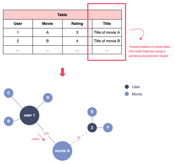
Figure 2 - Modeling the recommendation problem as a link prediction task, illustration by Lina Faik
In this context, the GNN model needs to be able to simultaneously learn embeddings for the user and movie nodes. To do this, one solution would be to take the GNN model compatible with a homogeneous graph and duplicate the message functions to work on each edge type individually. This process is detailed in the following figure.
This is the default architecture implemented in PyTorch Geometric. More precisely, the library provides an automatic converter that transforms any GNN model into a model compatible with heterogeneous graphs. The library also allows to build GNNs for heterogeneous graphs from scratch with custom heterogenous message and update functions. More information can be found here.
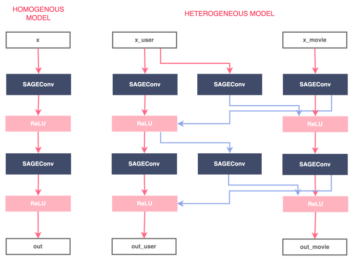
Figure 3 - Conversion of a regular GNN model to a GNN model adapted to heterogeneous graphs, illustration by Lina Faik, inspired by [3]
1.3 Link Prediction
The previous model allows us to train a model capable of generating the embedding of two nodes of different types.
How can these embeddings be used for link prediction?
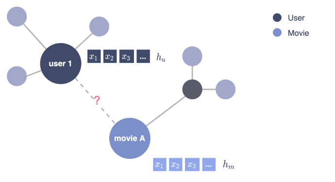 Figure 4 - Modeling the recommendation problem as a link prediction task, illustration by Lina Faik
There are two options:
Option 1. Train an additional linear model that takes (as an input) the concatenation of the user and movie embeddings to predict the rating. This is the approach implemented in the application part below.
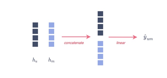
Figure 5 - From Node embeddings to link prediction (option 1), illustration by Lina Faik
Option 2. The other alternative consists of either:
- Computing a simple dot product, provided that the dimensions of both embeddings are the same and that the output is one-dimensional (e.g., predict whether the link exists or not):

- Learning a trainable matrix W = (W¹, …, W^k) so that:

You can find here the final code of the GNN model:
2. Application to Recommender Systems
This section describes the methodology used and discusses the results.
2.1 Methodology
✔️ Data
The data consists of the heterogeneous rating dataset, assembled by GroupLens Research from the MovieLens website. It contains two types of nodes: “user” and “movie.” A user node is linked to a movie node if he has rated the movie. The link is then labeled with the rating he gave.
Here is a short description of the data:

✔️ Model Evaluation
As shown in Figure 5, users tend to give ratings between 3 and 4 more frequently than other ratings. To this into account when training and evaluating the model, a weight is associated with each rating as follows:

where c_k is the number of occurrences of the rating k.
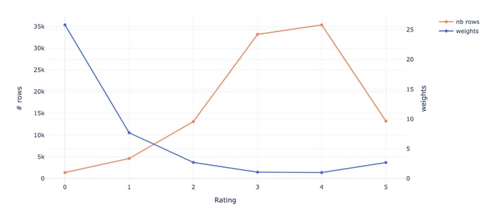
Figure 6 - Distribution of the ratings and associated weights, illustration by Lina Faik
In this context, the RMSE is weighted as follows:

✔️ Learning Framework
The data is divided into three:
- Training set (80%)
- Validation set (20%) used to choose the best combination of the model hyperparameters
- Test set (10%) used to compare the performance of the models
In order to measure the robustness of the results, the splitting was repeated five times. The graphs show the mean and the variance of the values.
2.2 Benchmark
Using this methodology, two different GNN models were tested, one using SAGEConv and the other GATConv.
To assess the performance of those graph-based models, the results are compared with a naïve algorithm and collaborative filtering standard models either based on KNN or matrix factorization.
1. A naïve algorithm: It draws random values from a normal distribution whose parameters μ and σ, are the ratings mean and standard deviation.
2. KNN-based algorithms
- It consists of computing the similarities between users (or movies) based on the ratings they previously gave (or received).
- The rating a user would give to a movie is then predicted as a weighted average of the ratings of the K most similar users (or movies) as follows:

- Other variants of this model exist as well. For more information about the implementation, you can read the library doc about KNN-based algorithms and similarity metrics.
3. Matrix factorization-based algorithms: Singular Value Decomposition (SVD)
- The model relies on a double-entry matrix representation of the problem: The rows correspond to the users, the columns to the movies, and the values are the ratings that the users have attributed to the movies.
- The model is then used to shrink the space dimension and thus reduce the number of features. In order words, they manage to map each user and each movie into a smaller dimensional latent space.
- The algorithm minimizes then a loss function which is the square error difference between the product of the user and movie new vectors and the true rating. Regularization terms can be also added to avoid overfitting issues.
For more information about the implementation, you can read the library documentation about SVD and SVD++.
2.3 Results
The results are presented below. For the sake of readability, only the best variants of each model were kept: KNN with Zcore for the KNN-based model and SVD for matrix factorization-based algorithms.
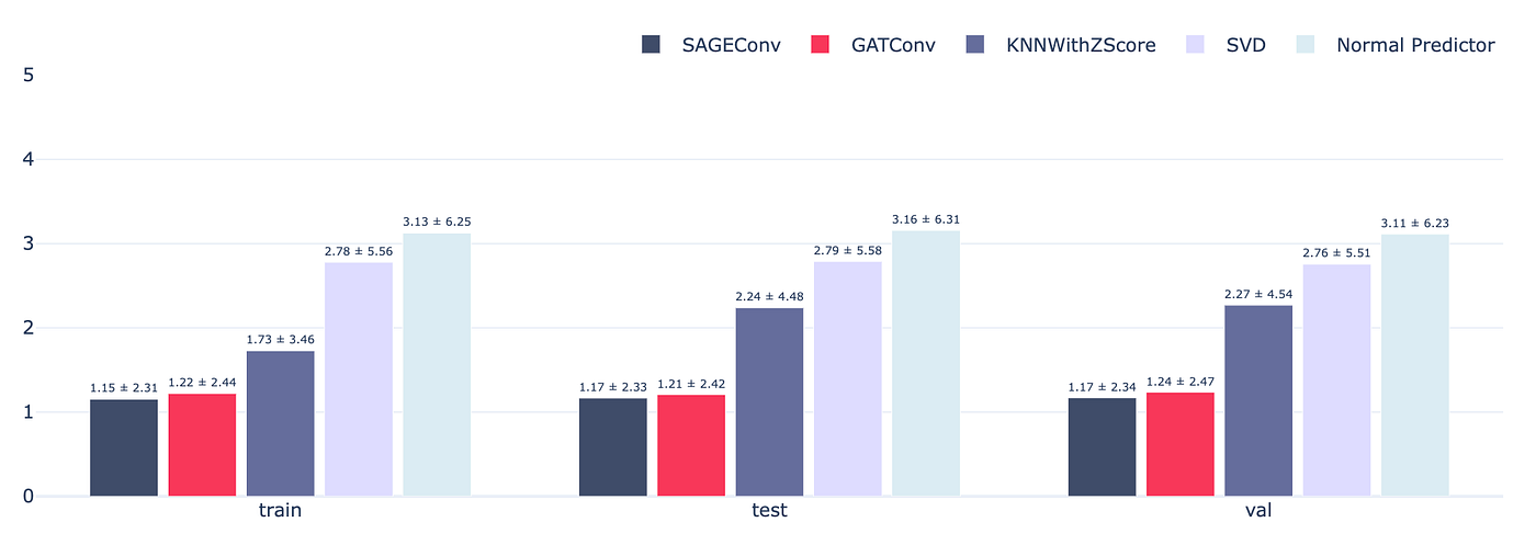
Figure 7 — Performance of the models in terms of weighted RMSE
The results show that graph-based models perform better than SVD. SVD tends to overfit the data and is therefore not able to generalize well.
Note also that there are no significant differences between GAT and GraphSAGE convolutions. The main reason is that GAT learns to give more or less weight to the neighbors of each node and is therefore somehow similar to the sampling strategy of GraphSAGE.
Nevertheless, GATs have also several issues compared GraphSAGE as mentioned in the first section. Among them is the fact that they are a full-batch model, they need to be trained on the whole dataset. Moreover, the attention weights are specific to each node which prevent GATs from generalizing to unseen nodes.
3. Key Takeaways
✔️ GraphSAGE convolutions provide a general inductive framework that relies on the same mathematical principles as GCNs but with a sampling mechanism. This enables GraphSAGE to efficiently generate node embeddings on large graphs or / and fast-evolving graphs.
✔️ Working with heterogeneous graphs brings an additional layer of complexity. A solution would be to take the GNN model used for homogeneous graphs and duplicate the message functions to work on each edge type individually as shown in Figure 3.
✔️ Link prediction refers to the task of predicting the existence or a characteristic of the relationship between entities within a network. To do so using a graph-based model, one option is to train a linear model that takes as input the concatenation of embeddings.
✔️ The application to the use case of movie recommendation shows that graph-based models perform better than the well-established collaborative filtering approach, SVD.