


If you have spent some time training machine learning models on large datasets, chances are that you faced some hardware limitations and had to cut away some of your data. In this blog post, we study the impact of training ML models on a (random) selection of the dataset and show that over six datasets of varying size, you can retain at least 95% of the performance by training a model on only 30% of the data.

Created with AI
In a second blog post, we’ll show how to leverage advanced data selection methods to get the most out of your data budget.
When Keeping All Data Is Not an Option
Many industrial applications (banking, retail, etc.) rely on extremely large datasets and training ML models on such datasets has to confront memory and time constraints due to hardware limitations. These issues are typical in applications where historical data is periodically collected and it is critical to train ML models on both past and recent data.
One option is to perform distributed training with Spark, for example, but when the required infrastructure is not in place or if the desired model is not supported by MLLib, the only viable solution is to select a subset of data that complies with our budget in terms of memory and training time constraints.
Working with large datasets also makes hyperparameter search, the process of tuning some model parameters before the actual training, extremely tedious, as it involves hundreds or thousands of individual model trainings on fractions of the full training set. While classical grid-search is extremely slow on large datasets, advanced search strategies, such as Hyperband [1], leverage small random selections to discard poor configurations of hyperparameters (HP) early in the process.
If data selection is necessary in many real-life applications, what is the best approach to select a relevant portion of my dataset without losing too much information?
Random Sampling: Training Models on Less Data
Thinking of selecting samples, the first natural method is random uniform sampling. The learning curves based on random sampling have been widely studied and published for many tasks, for instance a large database for tabular scikit-learn models (with default HPs) is available in LCDB [2].
If we consider three large datasets from LCDB (poker, covertype and codrna), we can observe three different situations (figure below), where the model is still learning (poker), the accuracy curve is flattening (covertype), and the learning curve is already flat (codrna).
Now, imagine we are ready to accept a 5% drop of accuracy with respect to the final accuracy, obtained using the entire training set. Observing where the learning curves cut the horizontal black line of the acceptable drop, we see we can reduce the amount of data used down to 36% (poker), 16% (covertype), and 5% (codrna).
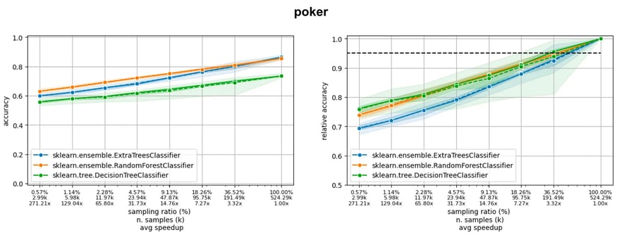
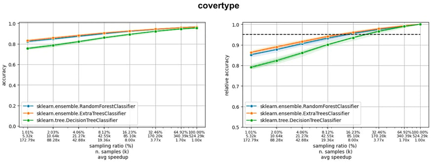
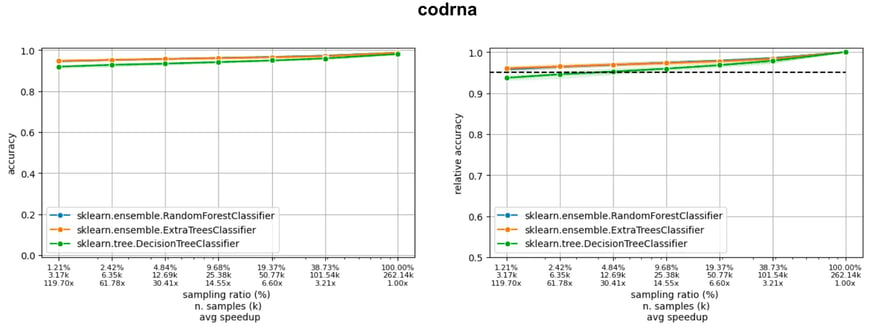 Learning curves of three models on three datasets in the LCDB database: the dotted line indicates a 5% drop with respect to the performance when training on the entire dataset.
On average across models, this would correspond to a training speedup from 5x to 140x, as displayed below. This figure captures the situation of retaining 95% of the final accuracy: The central plot y-axis shows the speedup with respect to the total fit time (annotated inside the bars), while the rightmost plot y-axis indicates the necessary portion of the entire dataset (the lower the better, full dataset size annotated inside the bars). The training speedup depends on the model scalability, for instance a logistic regression has a smaller speedup than a random forest for the same portion of the training set.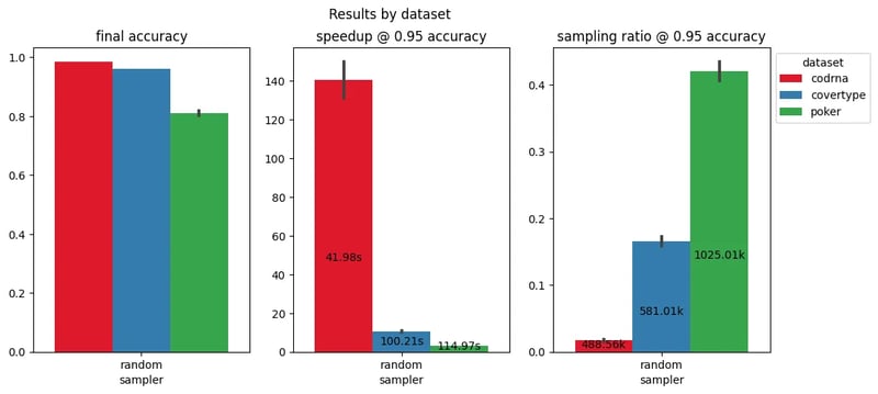
Speedup and sampling ratio corresponding to a 5% drop of the final accuracy (averaged across three ML models) on three datasets in the LCDB database.
Random Sampling: The Case of XGBoost
In order to have a look at the learning curves of better performing ML models for tabular data, such as XGBoostingClassifier, we realize our own benchmark on six datasets containing from 10,000 to 10 million samples (293/covertype, flight-delay-dataset, higgs, metropt_failures, tabular-playground-series-sep-2021, user_sparkify_event_data). We apply HP optimization before training and observe robust metrics, such as AUC and F1 score (instead of accuracy), to take into account imbalance in our data.
Let’s first have a look at how the performance of a XGBoosting classifier drops when training on various portions of data. At this end, we consider one single dataset with 10 million rows, metropt_failures, and simulate other six smaller datasets by taking portions of it. For instance, the dataset in blue consists of 10,000 samples from the same initial dataset, metropt_failures. From the figure below, you can see that the larger the dataset, the less pruning the training set will affect the performance.
The relative AUC is the ratio of the AUC obtained training the model on a subset of data and the regular AUC training the model on the entire dataset. For instance, training on 5% of a dataset with 10 million samples (pink line) lower the AUC to the 95% of the final AUC, while taking the 5% of a dataset with 50,000 samples (yellow line) will pull the AUC down to 85% of the final AUC.
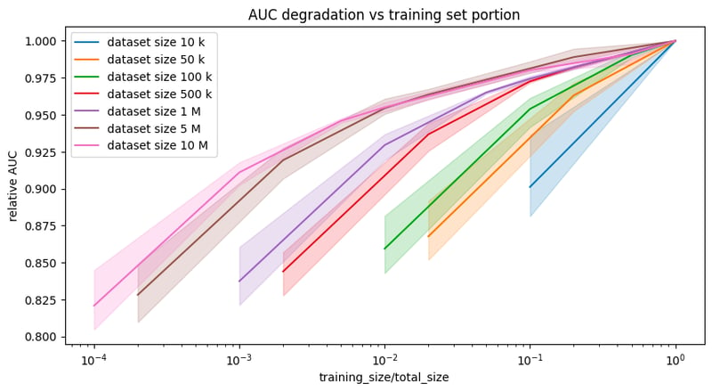
Relative AUC (AUC of model trained on a subset divided by AUC of model trained on the entire dataset) curves for datasets of different sizes. The larger the total size the less the impact of training on subsets on final performance is.
In spite of the peculiarities of each dataset (figure below), we always get the same diminishing return pattern. Even considering different models (XGBoosting, MLP, logistic regression), if a 5% drop of the final F1 score is acceptable, we can limit the training size from randomly sampled 1% to 30% of the entire dataset, and thus obtain from 10x to 500x speedup in training time.
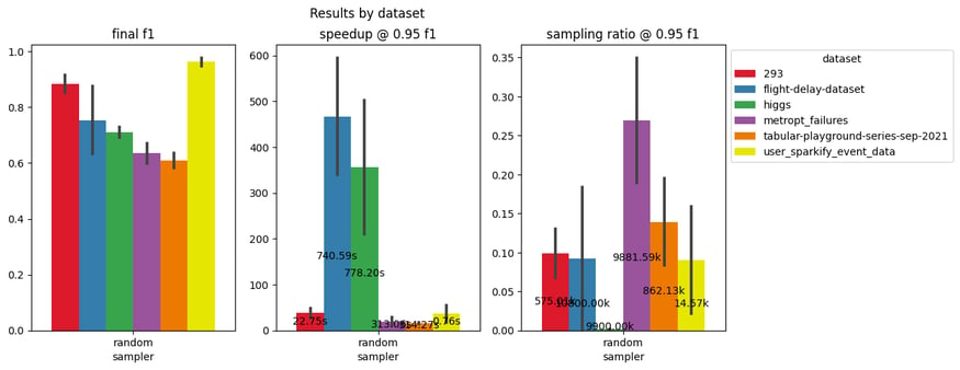
Speedup and sampling ratio corresponding to 5% drop of the final accuracy (averaged across three ML models) on six industry-like datasets (up to 10M rows).
For the specific case of XGBoostingClassifier, the average speedup across datasets is about 100x, as displayed in the figure below, where the y-axis of the central plot shows the speedup with respect to the total fit time (annotated inside the bars).
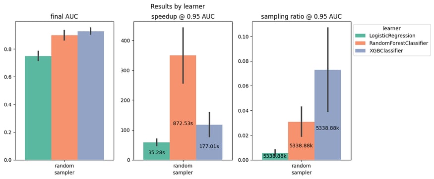
Speedup and sampling ratio corresponding to 5% drop of the final accuracy (averaged across six datasets) for three ML models.
Instead, hyperparameter optimization, which requires fitting hundreds or thousands of ML models before the final training, would take days and this is when these speedups become interesting.
Random Sampling: Tuning Hyperparameters on Less Data
Data selection offers a way to accelerate HP search, training the models with different configurations of HPs on small randomly sampled portions of the dataset. We are implicitly making an important assumption here: Whether we use small subsets or the entire dataset for training models during HP search, we’ll end up finding the very same best configuration.
In other words, we hope that, if configuration C1 is better than configuration C2 in the regular HP search, we also find that same relation, C1 better than C2, when doing an approximated HP search on small splits. Regardless of the dataset size, the relative performance of the configurations is roughly maintained, even if the performance metric will likely be higher (for both C1 and C2) in the regular HP search than in the approximated HP search, because the latter trains on less data models that will thus have lower quality.
A simple experiment [3], tuning an SVM classifier to classify MNIST digits, compares the performances (validation errors) of approximated HP grid search using 1/128, 1/16, 1/4 of the entire training set with the regular HP grid search on the entire dataset (figures from left to right, from 391 to 50.000 samples). The search is realized over a grid of 10x10 values in the logspace for the two hyperparameters, C and gamma.
We can easily observe that the best configurations (in blue) stay roughly the same regardless of the training size. To give an idea of the process length, on our machine (Intel Xeon E-2288G CPU @ 3.70GHz, 8 cores, 64 GB RAM) the full HP grid search takes around three hours, while the approximated search on 1/128 of the data takes 40 seconds, thus the speedup in HP tuning is 269x.
Although we don’t know how this can generalize to other models and datasets, still it’s encouraging towards using approximated HP search.
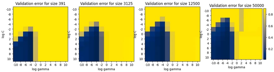
Validation error for 10x10 configurations of SVM hyper-parameters gamma and lambda. The HP search is performed on subsets of MNIST dataset of size 1/128, 1/16, 1/4, and the entire dataset from left to right.The subsets are randomly sampled.
The assumption that two configurations can be ranked even using small datasets is at the foundation of Hyperband [1] advanced HP search technique, whose authors point out that the closer in performance two configurations are, the more budget (larger size) we need to select the best between them.
We have seen that with uniform sampling, we can already realize interesting speedups, with an information loss that is acceptable for many applications. Nevertheless, there is a known limitation with random sampling: When dealing with under-represented subpopulations, like in imbalanced classification, it might miss minority or long-tail samples.
Can we do better than random sampling? And what does it mean concretely selecting a better portion of the dataset?
Learning Curves: Predicting the Effect of More Training Data
The learning curve of an ML model, or how its performance scales with the dataset size, gives interesting insights on the complexity of the task and on the effect of additional training data. It is good practice to compute the first points of this curve, training models on small (randomly sampled) training sets first. The shape of the obtained curve, as well as the variance of the performance as the training size increases, are indicative of what is left to capture and can support the decision of dismissing more training data.
There is empirical evidence that learning curves roughly scale as power laws, both for classical tabular models and for neural nets [4, 5]. ML researchers designed selection methods meant to identify partitions more representative than simple random splits, so that the scaling law of the performance increases faster. The steeper the curve, the smaller the dataset size at which we reach a given accuracy, the more effective the data selection is, as illustrated in this figure.
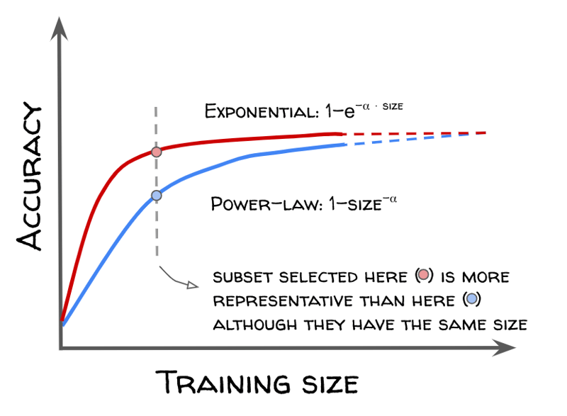
ML models learning curves generally follow power laws, while advanced selection techniques under research target faster exponential scaling.
With the hope of overcoming the limitations of random sampling, but also with the dream of breaking learning curves beyond power law scaling (models that learn faster with less data), researchers designed more advanced selection techniques that go by the name of active sampling, the topic of the next blog post.
Conclusion
Distilling very large datasets into smaller datasets for training ML models might be necessary because of resource constraints. A simple and fast way to do so is randomly selecting small batches, but don’t worry, it’s likely that your ML model’s performance will be reduced much less than you think: Over six datasets of varying size, you get 95% relative performance, training an XGBoosting model on only at most 30% of the training set.
With this article, you should now have an idea of the typical power-law scaling of the ML models learning curves and, if this sparked your interest, stay tuned to learn about non-random selection methods designed to learn faster with less data.