


In the first article of this three-part series, we highlighted preparing a dataset for machine learning (ML), which included data cleaning, feature selection, and feature handling and engineering. Now that the prep work is out of the way, we’re back to dive into actually building the model and evaluating it. We’ll cover interpreting the model in the next and last article of the series.
Building the Model
The first model you build should be a baseline, meaning a model that is straightforward but with a good chance of providing decent results. Building baseline models is fast and in many cases, it can get you 90% of the way to where you need to be. In fact, a baseline model may be enough to solve the problem at hand — with an accuracy of 90%, should you then focus on getting the accuracy to 95%? Or would it be a better use of time to solve more problems to 90% accuracy? The answer depends largely on the use case and business context.

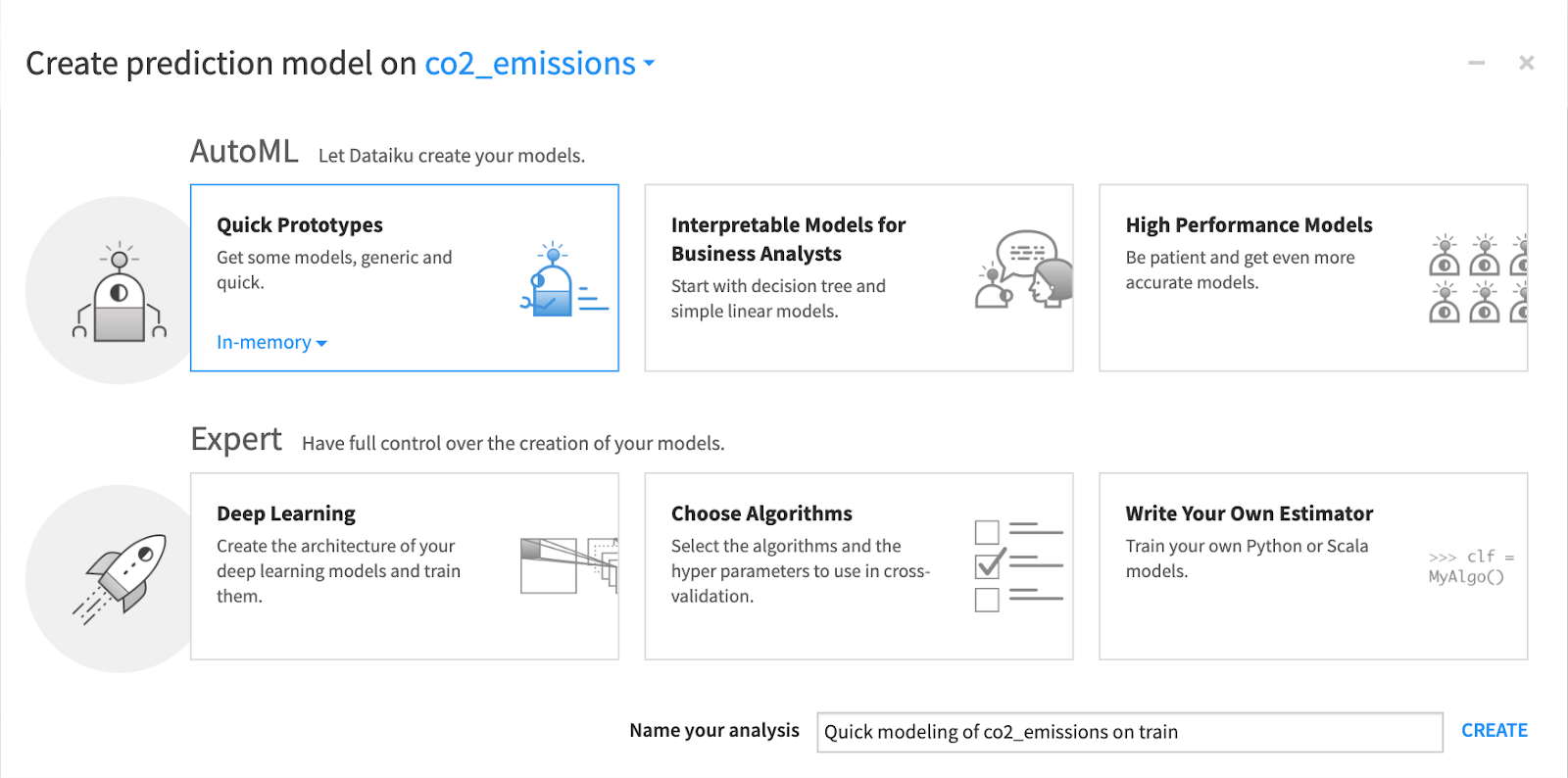
AutoML is a tool that automates the process of applying machine learning and can make quick, baseline modeling simple — even experienced data scientists use AutoML to accelerate their work. For example, in Dataiku, users can select between the AutoML mode where the tool makes a lot of optimized choices for you and the Expert Mode where you can control the details of the model, write your own algorithms in code, or use deep learning models. Note that in the AutoML mode, we’ll still be able to define the types of algorithms Dataiku will train. This will let us choose between fast prototypes, interpretable models, or high performing models with less interpretability.
Designing the Model
With Dataiku AutoML, you’ll still need to make a few decisions when creating your model (even for fast prototypes):
- Select a target variable. Since we are going with a supervised learning model, we need to specify the target variable, or the variable whose values are to be predicted by our model using the other variables. In other words, it’s what we want to predict. In the case of our Haiku T-shirts project, the variable we want to predict is the expected revenue that will be generated by new customers in the coming month.
- Regression, or predicting a numerical value. As our objective is to predict the amount of revenue that will be generated by T-shirt sales to new customers, it makes the most sense for our sample model to choose regression as the prediction type. Alternatively, if we were to formulate a slightly different problem and target variable on the same Haiku T-shirts data, we could go with classification instead.
- Classification, meaning predicting a “class,” or an outcome, between several possible options. If, for instance, we want to determine whether new customers are likely to be “high spenders” (which can be defined, for instance, as anyone who has spent more than $50 on our products in one month), we could use two-class classification to predict whether a customer will be a high spender (class 1) or non-high spender (class 2). Since in this case, we have two possible outcomes, this would be two-class classification, but for another problem it might make sense to have more than two outcomes, in which case it would be multi-class classification.
Training on a Subset of the Data
When developing a machine learning model, it is important to be able to evaluate how well it is able to map inputs to outputs and make accurate predictions. However, if you use data that the model has already seen (during training for example) to evaluate the performance, then you will not be able to detect problems like overfitting.
It is a standard in machine learning to first split your training data into a set for training and a set for testing. There is no rule as to the exact size split to make, but it is sensible to reserve a larger sample for training — a typical split is 80% training and 20% testing data. It is important that the data is also randomly split so that you are getting a good representation of the patterns that exist in the data in both sets.
Selecting the Algorithm and Hyperparameters
Different algorithms have different strengths and weaknesses, so deciding which one to use for a model depends largely on your business goals and priorities. Questions you might ask yourself include:
- How accurate does the model need to be? For some use cases, like fraud detection, accuracy is critical. Others, like — say — a recommendation engine, don’t need to be as accurate to be successful and provide business value.
- Is interpretability important? If people need to understand how any individual predictor is associated with the response, it might make sense to choose more interpretable algorithms (e.g., linear regression).
- How much does speed matter? Different algorithms will take different amounts of time to score data, and in some business contexts, time is of the essence (even just a few fractions of a second — think getting a quote for car insurance). Decision trees are usually fast as well as accurate which makes them a good baseline choice.
It’s also important to understand the concept of libraries, which are sets of routines and functions that are written in a given language, making it easier to perform complex ML tasks without rewriting many lines of code. For example, Dataiku AutoML comes with support for four different machine learning engines:
- In-memory Python (Scikit-learn / XGBoost)
- MLLib (Spark) engine
- H2O (Sparkling Water) engine
- Vertica
Beyond choosing an algorithm, one other aspect of building an ML model is tuning hyperparameters. Hyperparameters are parameters whose values are used to control the learning process — think of them as the settings of the machine learning model. They matter because they control the overall behavior of a ML model, and tuning or optimizing hyperparameters can help your model perform better.
Performing hyperparameter optimization is really about searching for the best possible model you can find within your time constraints. One way to refine the search space is to study which hyperparameters are most important and focus on them. For a given machine learning task, it is likely that changing the values of some hyperparameters will make a much larger difference to the performance than others. Tuning the value of these hyperparameters can therefore bring the greatest benefits.
Finding the best combination of hyperparameters is really hard, and uncovering how to do so could be a topic in and of itself and is outside the scope of this guide. For a baseline model, AutoML helps by quickly honing in on the most promising potential hyperparameter optimizations, and therefore can help you build better models in a limited amount of time.
Evaluating the Model
You’ve connected to data, explored it, cleaned it, and created a quick model. Now what? How do you know if your model is any good? That’s where tracking and comparing model performance across different algorithms comes in.
Metrics Evaluation and Optimization
There are several metrics for evaluating machine learning models depending on whether you are working with a regression model or a classification model. It’s also worth noting that for most algorithms, you’ll also choose a specific metric to optimize for during the model training. However, that metric might not be as interpretable as some of the other evaluation metrics for actually determining how well a model works.
For regression models, you want to look at mean squared error and R-squared (R2)
- Mean squared error is calculated by computing the square of all errors and averaging them over all observations. The lower this number is, the more accurate your predictions were.
- R2 (pronounced R-Squared) is the percentage of the observed variance from the mean that is explained (that is, predicted) by your model. R2 always falls between 0 and 1, and a higher number is better.
For classification models:
- The most simple metric for evaluating a model is accuracy. Accuracy is a common word, but in this case we have a very specific way of calculating it. Accuracy is the percentage of observations that were correctly predicted by the model. Accuracy is simple to understand but should be interpreted with caution, in particular when the various classes to predict are unbalanced.
- Another metric you might come across is the ROC AUC, which is a measure of accuracy and stability. A higher ROC AUC generally means you have a better model.
- Logarithmic loss, or log loss, is a metric often used in competitions like those run by Kaggle, and it is applied when your classification model outputs not strict classifications (e.g., true and false) but class membership probabilities (e.g., a 10% chance of being true, a 75% chance of being true, etc.). Log loss applies heavier penalties to incorrect predictions that your model made with high confidence.
Overfitting and Regularization
We’ve mentioned overfitting in some of the previous sections, but at this point, it’s worth coming back to it in more detail as it can be one of the biggest challenges to building a predictive model. In a nutshell, when you train your model using the training set, the model learns the underlying patterns in that training set in order to make predictions.
But the model also learns peculiarities of that data that don’t have any predictive value. And when those peculiarities start to influence the prediction, we’ll do such a good job at explaining our training set that the performance on the test set (and on any new data, for that matter) will suffer. One remedy for overfitting is called regularization, which is basically just the process of simplifying your model or making it less specialized.
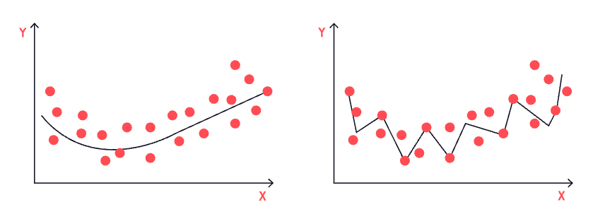
On the right is a visual representation of overfitting, or when a model is too well trained (compared to the model on the left, which is robust and a good fit, i.e., just right!).
For linear regression, regularization takes the form of L2 and L1 regularization. The mathematics of these approaches are out of our scope in this guide, but conceptually they’re fairly simple. Imagine you have a regression model with a bunch of variables and a bunch of coefficients, in the model y = C1a + C2b + C3c..., where the Cs are coefficients and a, b, and c are variables. What L2 regularization does is reduce the magnitude of the coefficients, so that the impact of individual variables is somewhat dulled.
Now, imagine that you have a lot of variables — dozens, hundreds, or even more — with small but non-zero coefficients. L1 regularization just eliminates a lot of these variables, working under the assumption that much of what they’re capturing is just noise.
For decision tree models, regularization can be achieved through setting tree depth. A deep tree — that is, one with a lot of decision nodes — will be complex, and the deeper it is, the more complex it is. By limiting the depth of a tree, by making it more shallow, we accept losing some accuracy, but it will be more general.
Stay tuned for the next article in this series where we dive into interpreting the model!