Machine learning model serving architectures

After months of crunching data, plotting distributions, and testing out various machine learning algorithms you have finally proven to your stakeholders that your model can deliver business value. Your model has to leave the comforts of your development environment and is ready to move to production to be consumed by the end user. Serving a model cannot be too hard, right? It doesn’t have to be. Selecting the right architectural serving pattern is paramount in creating the most business value from your model. In this blog we will discuss the most common serving architectures¹; batch predicting, on-demand synchronous serving and streaming serving. For the sake of argumentation, we will assume the machine learning model is periodically trained on a finite set of historical data. After reading this post you will understand what business requirements, quality attributes and constraints drive the decision for the serving architecture and will enable you to choose the architecture that best suits your use case.

_{1. Other serving architectures include; edge serving, federated learning, and online learning. Those are more advanced serving architecture warranting a blog post of their own.}

In this blog post we refrain from mentioning specific tools and technologies to avoid the rabbit hole of implementation details. Instead we focus on the principles that drive the discussion. There are many ways to implement each of the referred architectures and some of them may even be combined in hybrid forms. Many different factors influence the architecture around a machine learning model. The serving architecture provides a solid reference point for further discussions.

Glossary

Throughout this post some definitions will recur. These definitions are listed below for reference and to scope the discussion on the serving architectures in the respective paragraphs.

• Prediction
  A prediction is data generated by applying a function (the model) to input data
• Latency
  Latency is measured by the time it takes for a prediction to reach the user the moment it is requested. It is the time it takes for the “Reads predictions” (see figure 1) interaction to complete.
• Throughput
  Throughput is the number of predictions that can be made per unit of time e.g. 1000/second
• Staleness
  The staleness of a prediction is the time between the user requests a prediction and the time a prediction was computed. A prediction is as stale as the input data and model used to compute it.
• Time sensitivity
  Time sensitivity is defined as the value of your predictions as a function of staleness. If predictions are highly time sensitive, stale predictions have little value. Vice versa, predictions with low time sensitivity are valuable over a longer period of time.

How to choose your serving architecture?

The following questions drive the choice of architecture:

• What is the time sensitivity of my predictions?
  The frequency of input data ingestion constrains the level of time sensitivity that can be satisfied. A higher ingestion frequency means more time sensitive use cases can be addressed. This can be extrapolated to real-time data ingestion that allows us to serve the use cases with the highest time sensitivity. This shows the (data) infrastructure supporting you can constrain the serving architecture.
• How do the users interact with the predictions we serve?
  Understanding how your model is used helps understand the constraints of the environment your model runs in. Your users may need to provide input for the model to make its prediction. This often means your application is in the critical path of the user journey. This will have implications on your architecture.

Batch predicting

A batch prediction job is a process runs for a finite amount of time on a finite set of data. The process is triggered periodically. The bounds of the dataset are specific to the use case. Batch predictions are typically stored in an SQL table or in-memory database to serve with low latency. 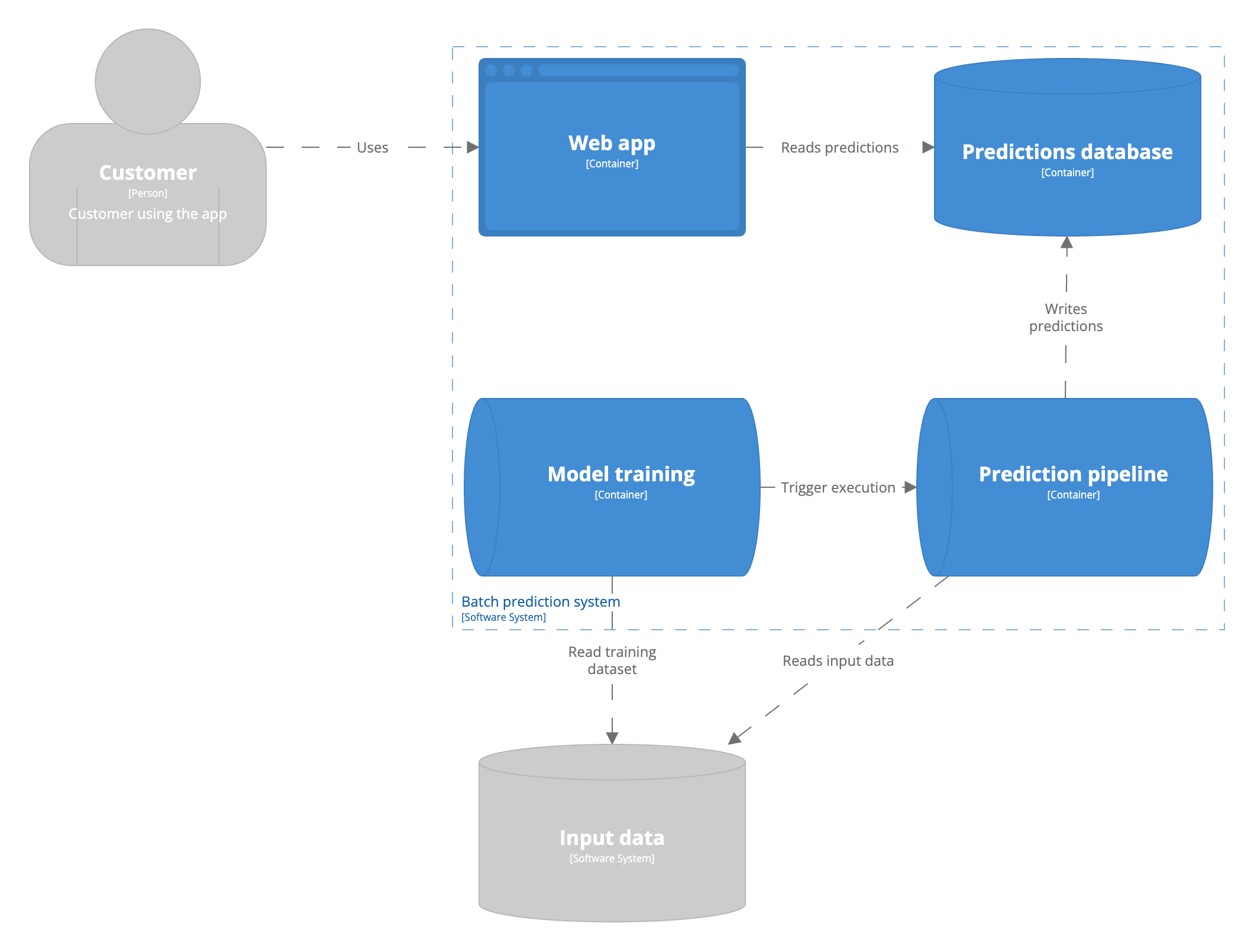Serving batch predictions is sometimes called asynchronous prediction. This means predictions are computed asynchronously from the user request. This causes a staleness in predictions served to the user. Everything that happened between computing and using the features is excluded from the prediction served to the user. For example, an e-commerce company may recommend products for users on their website. The recommendations are computed every few hours and served when a user logs in. All that happens within these few hours until the next run will not be reflected in the recommendations. This makes batch models less adoptable to change in user behaviour.

Serving predictions in batch is the simplest form of model serving. The serving architecture is technically similar to how a model is trained. Computing predictions in batch allows the team to inspect the predictions prior to exposing them users. This allows less mature teams to create trust in the predictions produced by a model. Distributed computation frameworks are commonly accessible to many organizations and individuals. They have been optimized over the years to process large volumes of data. Batch predictions are unsuitable when the domain is unbounded. The domain refers to all possible input values. Batch predictions run against a finite dataset, so it is unsuitable if there is no limit to all possible input values. For example, it is impossible to know all input images for an image classification model. Thus, you will never serve an image classification model in batch. Finally, batch computations can be used to reduce latency. You can pre-compute all predictions and serve them from a database when the user requests them if the prediction computation time is long.

Pros:

• Simplicity
• Maintainability
• High throughput
• Low latency

Cons:

• Time sensitivity
• Limited to bounded domains

On-demand synchronous serving

In this model serving architecture a model is hosted as a stateless web server and exposed over an HTTP or gRPC endpoint. This is referred to as synchronous serving, predictions are computed the moment a user requests it. The predictions are computed synchronously from the user’s perspective. The user cannot proceed with the application before the prediction is returned. The user provides a part or all of the input features in the request. The model can make use of additional batch features, or use both batch and streaming features. There is a distinction between models only using batch features and streaming features. It has implications on the serving architecture and infrastructure requirements. Both modes can experience challenges meeting latency requirements. Computing a model prediction can take long. This may violate the latency requirement because the prediction is computed when the prediction request is made.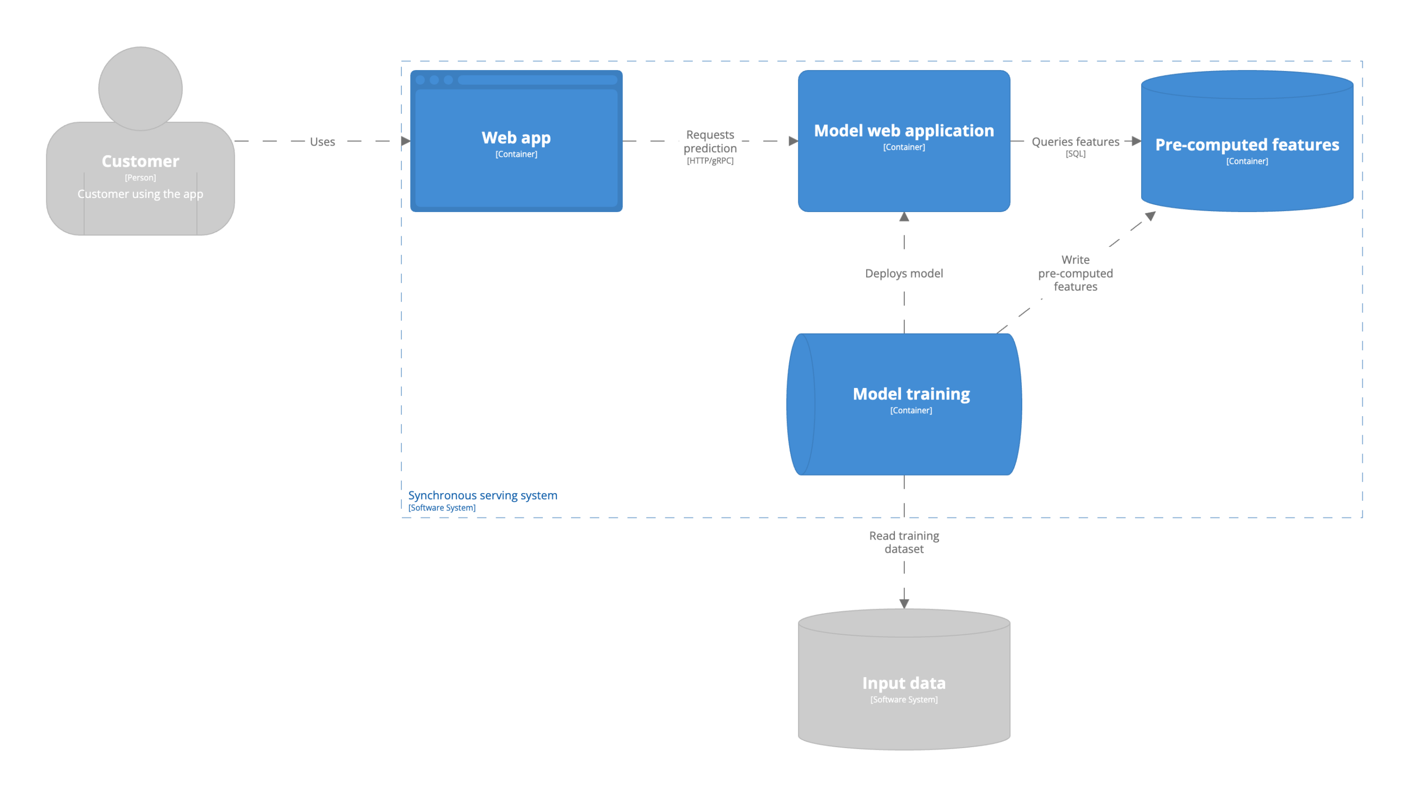

Batch features

Just like batch predictions, batch features are computed periodically. An example of a batch feature is the number of times a user has visited a website in the past month. Using batch features in models is recommended when the features change infrequently. The data availability of input data used to compute the model features dictates if your input features are batch features. If your input data is ingested into the data warehouse in batch, your features will be batch features. Your architecture is thereby dictated by the constraints of the environment you operate in.

Pros:

• Simplicity
• Unbounded domain

Cons:

• Time sensitivity
• Throughput
• Latency

Batch and streaming features

Streaming features are features that are updated in real-time with low latency. Using streaming features requires your company to support streaming data processing architectures. A streaming feature could be the items a user has browsed in the current session. As mentioned above, the model still runs as part of a stateless web server. Yet, the features the model uses as input to compute a prediction come from a database updated in real-time by streaming data pipelines. In these scenarios companies often make use of a feature store. The concept of, and requirements, for a feature store will not be discussed in this blog post. For simplicity we assume the feature store in the architecture reconciles batch and streaming features and provides the application with a unified interface to query both. 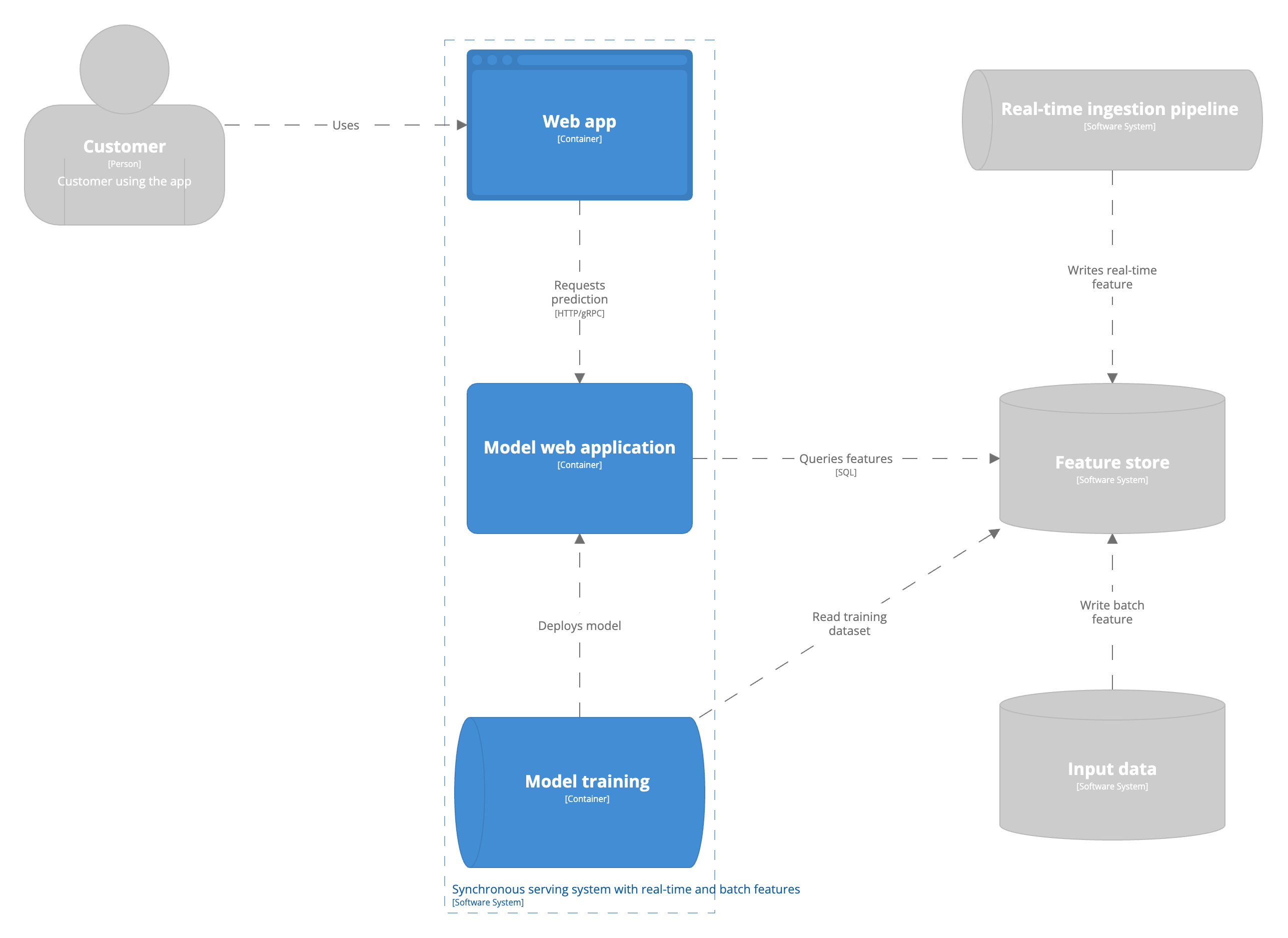The main advantage of leveraging streaming features is the ability to quickly adapt to changes in user preferences. You will always have the most up-to-date view of the world available to your machine learning model to make predictions on. Let’s go back to the earlier example of the e-commerce company. In the batch prediction example none of the user activity between the last run and the next run of the batch pipeline is captured in the prediction. The real-time data pipeline keeps track of the user interactions in real time and the model has access to these features through a feature store. Having access to the items a user has viewed during their current session allows our recommender to suggest more relevant products.

Pros:

• Unbounded domain
• Time sensitivity

Cons:

• Throughput
• Complexity
• Debuggability / traceability
• Latency

Streaming predictions

This serving architecture is referred to as asynchronous real-time serving. Predictions are computed on an infinite stream of input data with low latency. Hence, the real-time component in the definition in contrast to batch predictions. The predictions are computed asynchronously from the user’s perspective. Users do not directly request predictions. The predictions are served asynchronous from the interaction they have with the application. 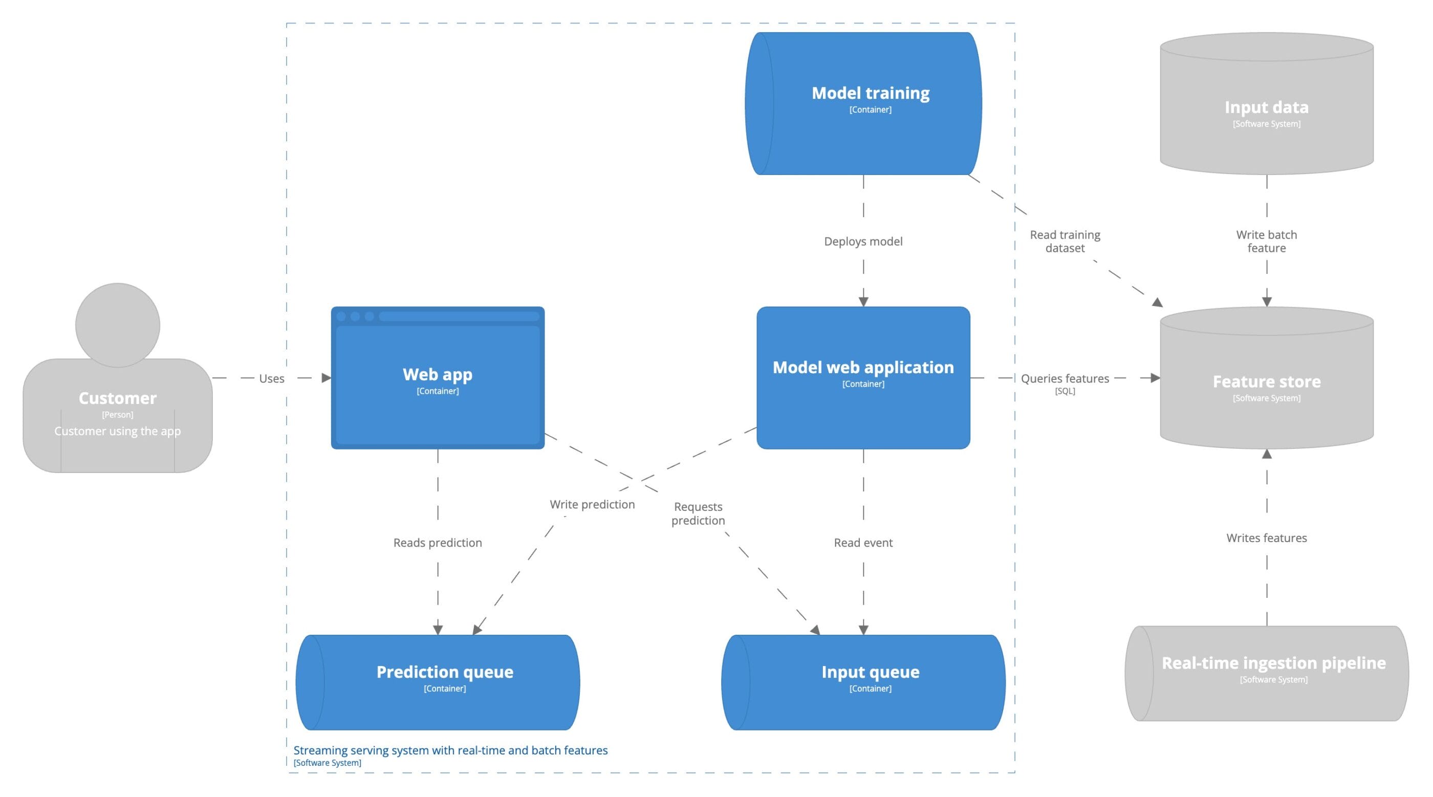It may seem as if moving towards streaming predictions is the ultimate goal to generate the most business value. However, as with all architectural decisions, it depends. Imagine you work at a bank and operate a prediction pipeline to identify money laundering. It involves multiple consecutive actions spanning weeks, months, or even years. Acting on the identification of a person as a money launderer is not immediate. Thus, running this pipeline every week or month in batch is enough.

Pros:

• Throughput
• Time sensitivity
• Robustness

Cons:

• Complexity

Example

Let’s illustrate with an example. Imagine you work for a bank. You have to classify transactions into categories to provide users insights into their spending. We still want users to be able to complete a transaction in case the classification fails. The classification of the transaction is not in critical path of the transaction, so the classification can be computed asynchronously.

Streaming predictions have two main benefits over synchronous serving; throughput and robustness. The trade-off is system complexity. Streaming predictions leverage message brokers to decouple the service requesting the prediction and the one serving the prediction. The introduction of the message broker increases the system’s fault-tolerance making the system more robust in face of adversity. The message broker makes the system more complex in terms of monitoring and maintainability.

Conclusion

In this blog post you learned what drives the decision for model serving architecture. You learned progressively complexer architectures. You saw different concrete use cases where the respective architecture provides value. The high-level architecture diagrams visualize the components that play a role in the machine learning system. You are now able to analyse the requirements for your project and choose the right model serving architecture.