
BigQuery is a serverless, highly scalable storage and processing solution fully managed by Google. It offers a lot of flexibility in computation and a variety of technology and pricing models. However, to leverage this platform and effectively utilize the infrastructure, adequate planning, monitoring, and optimization are required.
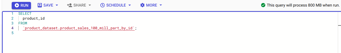
Estimating the cost impact of any query is fundamental to optimizing a project’s budget. For most query requirements (other than ones that use cluster), we can estimate the exact amount of data processed. The query validator in the Google cloud console validates the query syntax and provides this estimate. We can also use the bq command with ‘dry_run’ flag for estimation. With this information, we can calculate the query costs using Google Cloud Pricing Calculator.
How to Optimize Queries and Control BigQuery Costs
Query optimization is the process of defining the most efficient and optimal way to perform a query. Through query tuning, we can decrease the response time of the query, prevent excessive resource consumption, identify poor query performance, and reduce associated costs.
Set up custom quotas
Custom quota is not a query optimization technique per se. At the same time, setting quotas can prevent budget overrun and point us to potential optimization issues when there are multiple users and projects. We can set daily quotas at the project or user level.
Analyze audit logs
BigQuery Audit Logs help you analyze platform usage at the project level and down to individual users or jobs. These logs can be filtered in Cloud Logging or exported back to BigQuery, where you can analyze them in real time using SQL. Knowing where and when more resources and time are taken can help reorganize tasks and improve performance.
Run as few SELECT * queries as possible
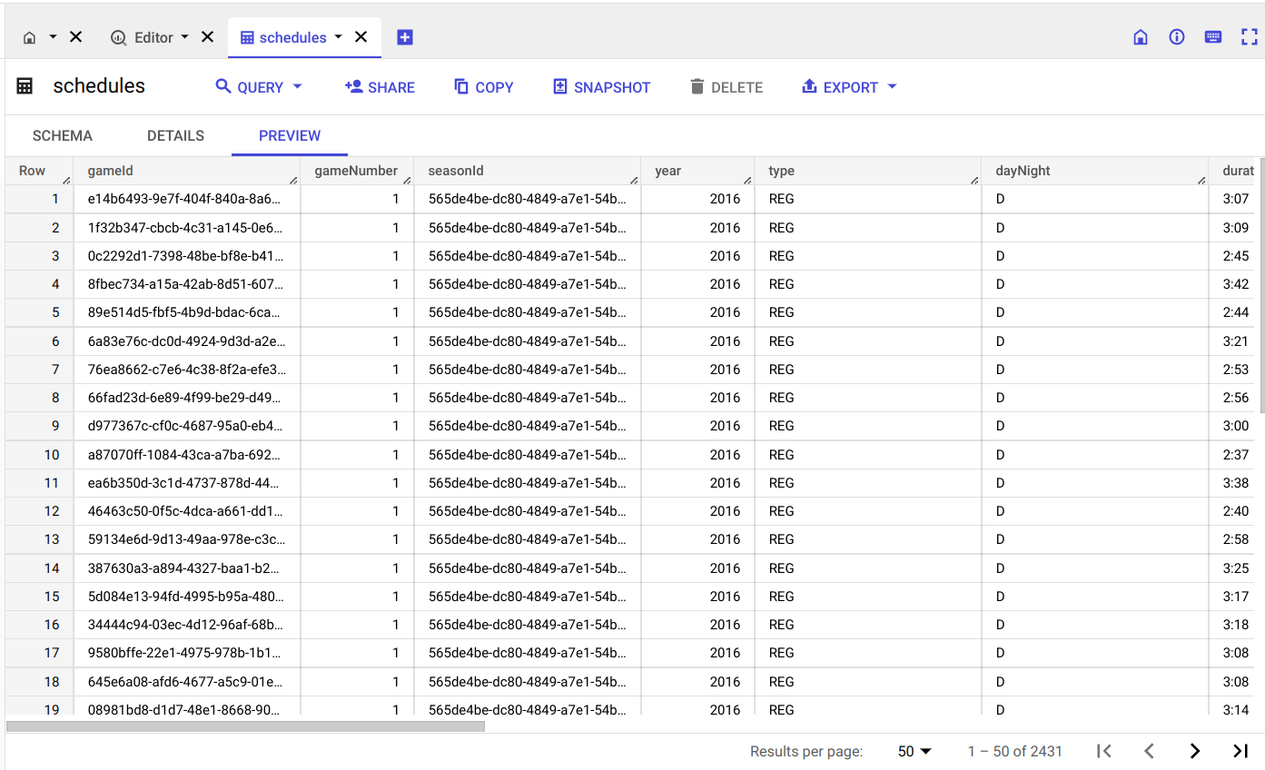
In your eagerness to explore new data, you may sometimes run too many SELECT queries, especially SELECT * statements, and exhaust the custom quota. When the need is to understand the data format such as various columns, it is better to use some of these techniques to preview data: (1) preview tab on the table details page in Google cloud console (2) ‘bq head’ command (3) tabledata.list method in the API. These preview modes are not chargeable.
Now, why is running SELECT * a bad idea?
BigQuery is a columnar database, unlike traditional row-based databases. If the query is to retrieve only 2 columns out of 100 columns, a row-based database will scan all 100 columns of each row to extract the 2 columns while BigQuery will only read the relevant 2 columns, which makes the query faster and more efficient.
If there is a large number of columns to be read, use SELECT * EXCEPT instead of SELECT *. If you still need to get all the columns but only a subset of data, it's ideal to store the table in partitions and read only the relevant partition or store materialized results in a destination table and read that table.
Use partitioning and clustering wisely
Partitioning and clustering both serve to reduce cost by narrowing down the section of data to be read for query execution.
When a query involves filters against partition keys, BigQuery filters out the irrelevant partitions at storage. Partitions are effective on tables that are bigger than 1 GB and are better for low cardinality fields. There can be up to 4000 partitions in a partitioned table. Do avoid data skew (uneven distribution of data in partitions) as it can impact query performance.
A clustered table separates data into blocks and then sorts the data in each block based on the column (or columns) that we choose and then keeps track of the data through a clustered index. While querying, the clustered index points to the blocks that contain the data. Thus irrelevant data scanning is avoided. Clustering is effective on tables bigger than 1 GB and having high cardinality fields. If done on multiple fields, you can specify up to 4 columns and they should be in descending order of cardinality. If you need more columns, then consider combining clustering and partitioning.
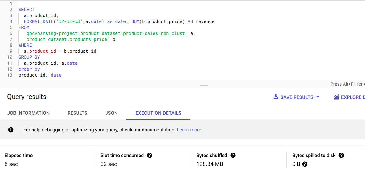
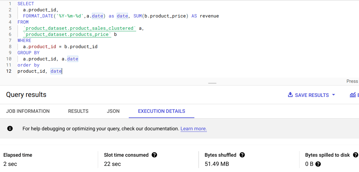
The example below shows the performance gains from clustering. On a clustered table, query execution took only 2 seconds compared to 6 seconds in a non-clustered table, which is a 67% gain.
Set maximum bytes billed
You can use the 'Maximum bytes billed' in the Query settings of the query editor to limit the number of bytes billed. If the query execution estimate goes beyond the limit, the query will fail. Note that for clustered tables, the query editor often overestimates the number of bytes required. Thus, queries that require fewer bytes than the limit set will fail to run.
Set expiration time for datasets and tables
Tables will get deleted after their expiration time and you will not have to pay for the storage. This will also help prevent the overgrowth of datasets and tables in your project.

Apply LIMIT on clustered tables
Remember that using LIMIT on non-clustered tables does not help reduce cost as the entire data needs to be read to generate query results. But applying LIMIT on clustered tables benefits cost reduction because scanning stops when the required number of blocks are scanned.
Set budgets and alerts
You can create budgets on GCP and monitor your actual spending against your planned spending. By setting up budget threshold rules and budget alerts, you can stay informed about how well or carelessly you are spending against your set budget. You can also use the budgets to automate cost-control responses.
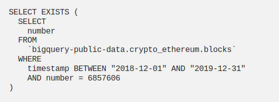
Use EXISTS() instead of COUNT()
Do you often check for the value in a table using COUNT()? If the exact count is not important, it is better to use EXISTS() because the query exits from execution as soon as a match is found. Smaller data scan results in reduced costs.
Trim data early and often
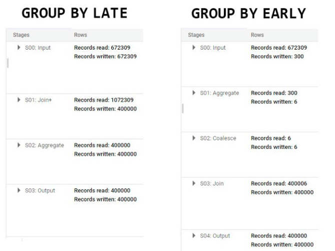
In BigQuery, multiple machines are used to execute a query. To get the correct results, individual outputs are reshuffled. Reduced shuffling can help with query performance. Filtering functions should be applied as early as possible to reduce the data shuffled and resource wastage.
For example, Applying GROUP BY clause within the innermost query and a JOIN operation in the outermost query helps reduce the data volume required to perform the JOIN operation. The below example demonstrates how performance improves when the GROUP BY operation is performed early in the query.
Take advantage of caching to reduce data scans
BigQuery has a cost-free, fully managed caching feature for queries. When we execute a query, BigQuery automatically caches the query results into a temporary table, which lasts for up to 24 hours. When a duplicate query is run, BigQuery returns the cached results instead of re-running the query, saving us the extra expense and compute time.
Use MATERIALIZED VIEWS for redundant queries
Use MATERIALIZED VIEWs (MVs) to take advantage of caching for faster and cheaper queries. MVs are snapshots of data saved on disk. BigQuery automatically refreshes and maintains MVs, so it's hassle-free. You can choose to query the MV or the base table; the query will be automatically redirected to MVs when applicable. MVs can only be created on native tables. Only inner joins can be applied on MVs, other joins are not supported.
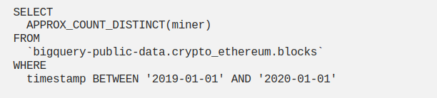
Use approximate aggregate function
When there is a large dataset and an exact value is not required, approximate aggregate functions should be used. Unlike the usual brute-force approach, approximate aggregate functions use statistics to produce an approximate result. The expected error rate is around 1~2%. Since we are not performing a full table scan, approximate aggregate functions are faster and highly scalable in terms of memory usage.
Perform resource-intensive operations on top of the final result
SQL operations like ORDER BY, Regular expressions (REGEX), Aggregate functions, etc. are expensive.
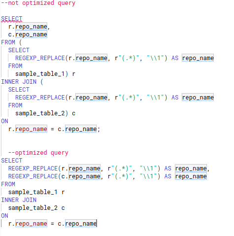
ORDER BY has to compare every row in order to organize rows in sequential order. Similarly, Regular expressions and Aggregate functions have to iterate over the whole data in order to get the results. The source table from which we are trying to query the result might have a huge volume of data. The queries may contain multiple subqueries, WHERE conditions, and GROUP BY clauses that reduce the data. It is always helpful to execute expensive operations on this reduced data than the original larger dataset.
Here's an example of how we can convert a non-optimized query into an optimized one.
Replace self-joins with window function in queries
Self-joins are used to find related rows in a table and perform aggregate operations on the result. While self-joins provide flexibility, they are inefficient and can create an SQL antipattern. This is because they multiply the number of output rows or force unnecessary reads, impacting query performance. As the table gets bigger, the problem gets worse.
A window function is a substitute for self-joins in most cases. It applies calculation across a set of rows related to the current one. It does not group the rows for an aggregate operation and maintains their separate identity. Thus it is able to access more than just the current row of the query result, making it an efficient approach.

Use INT64 data type as ORDER BY clause and JOIN key
Always go for INT64 data type in JOINs and ORDER BY clause instead of a STRING data type. INT64 is a simple array of 64-bit integers, and therefore cheaper to evaluate when compared to STRING. In contrast to traditional databases, BigQuery does not index primary keys, so the wider a key column is, the longer it will take to compare them. Therefore, using INT64 columns as join keys and order by columns can improve query performance.
Avoid multiple evaluations of the same CTEs
Common Table Expressions (CTEs) are temporary named result sets that can be referenced in SELECT, UPDATE, INSERT, or DELETE statements. They are temporary because they cannot be saved for future use and will be lost as soon as the query execution is complete. They are used to simplify complex queries by splitting them into simpler ones and can be reused within the same query. Referencing a CTE multiple times in a query leads to increased resource consumption and makes the internal query more complex. Instead, we can store the result of a CTE in a scalar variable or a temporary table depending on the data that the CTE returns. The temporary table storage in BigQuery does not incur any charges.
Optimize join patterns and use filter methods to avoid data skew
Data skew occurs when BigQuery distributes data unevenly for processing. Uneven distribution happens when a partition key value occurs more often than any other. This causes an imbalance in the amount of data sent across slots.
Make use of approximate aggregate functions such as APPROX_TOP_COUNT to evaluate partition keys. A query consisting of a join operation should be ordered in such a way that the table with the largest number of rows is placed first, followed by the remaining tables in the order of decreasing size.
When we have a large table on the left side of the JOIN and a small one on the right, a broadcast join is created. A broadcast join sends the data from the smaller table to each slot that processes the larger table, causing performance degradation. Therefore always perform broadcast join first.
Use the BigQuery slot estimator to choose the right pricing model
BigQuery offers two types of pricing models, on-demand and flat-rate. In on-demand pricing, charges are calculated based on the volume of data processed by the queries. Failed queries and queries loaded from cache are not charged. In flat-rate pricing, users have to pay a fixed charge regardless of the amount of data scanned. This is suitable for users who are expecting a predictable monthly cost within a specified budget.
It is always better to start with the on-demand pricing model. We can use the BigQuery slot estimator to understand our on-demand slot consumption. Slot estimator can be used for both flat-rate and on-demand billing models and it helps us in understand the possible impacts of moving from on-demand to flat-rate.
To address the occasional rise in demand, we can make use of the Flex slot functionality. Slots can be purchased for as little as 60 seconds at a time.
Use INFORMATION_SCHEMA for job monitoring
INFORMATION_SCHEMA are views created by BigQuery, which contain the metadata information on BigQuery objects. The INFORMATION_SCHEMA can provide comprehensive information on tables, their consumption, and performance. This can help us decide our optimization strategies.
Querying against INFORMATION_SCHEMA incurs a cost and that varies depending on the pricing model we choose. A minimum of 10MB data processing charge applies to on-demand pricing. For flat-rate, the cost will depend on the number of slots purchased. The INFORMATION_SCHEMA queries are not cached, so each query is charged separately.