

Graph Neural Networks (GNN) have proven their capability in traffic forecasting, recommendation systems, drug discovery, etc., with their ability to learn from graph representations. What I'm going to do here is take you through the working of a simple Graph Neural Network and show you how we can build a GNN in PyTorch to solve the famous Zachary Karate Club node classification problem.
The Zachary Karate Club is a dataset created by Wayne W Zachary based on his study of the social network of a university karate club. Following an argument between the instructor and the administrator, the karate club broke into two. Zachary represented this data as a graph, with nodes representing the members and edges representing the relationship between the members outside the club (see below graph). Node 1 represents Mr. Hi, the karate instructor; Node 34, the administrator John A.
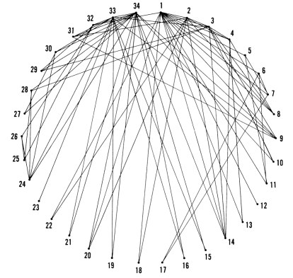
We have to identify the members of the two groups by analyzing whether the members met outside of the karate club. This problem is typically solved with network analysis techniques, but here we will use a GNN.
I will walk you through the whole GNN pipeline from creating a graph dataset to evaluating the model and we will explore how far our GNN model is able to learn from the patterns inside the graph with minimal supervision.
How Graph Neural Networks Work
Graph Neural Networks are a class of neural networks that can learn and optimize from graph data. There is a lot that can be learned from graphs because they help represent complex relationships between data entities more meaningfully. If we try to represent a graph in a Euclidean space like a vector, we will lose critical information that might be useful for downstream tasks. So graphs are represented as a collection of vectors. Neural networks like CNN and RNN do not have the capability to learn from such data but a Graph Neural Network can.
Generally, graphs contain four types of information: Node, Edge, Connections, and Global context. All this information can be represented as individual vectors. "Connections" is a sparse vector that grows exponentially with the number of nodes. This will cause higher resource consumption while training. So Connections are generally represented with an Adjacency list and the other information with vectors.
A graph Node is not only represented by its own features but by its neighborhood as well. This means a single node’s representation should somehow reflect neighborhood information like the connected nodes, type of edges connecting the nodes, etc.
Message Passing
One approach GNN takes to learn neighborhood information is message passing. The idea is that, in each message passing iteration, each node receives messages from its neighbor, and the node embedding gets updated with these messages. This works in three steps:
- Message Propagation - Each node receives the node embedding of its neighbors as messages.
- Aggregation - The received messages are aggregated using an order invariant function like sum or average. The order invariant function is used because all neighboring nodes are similar and the order in which they are selected should not change the calculation.
- Update - The current representation of each node is updated by passing the current node embedding and the aggregated messages through a neural network.
The output of this message passing layer can be used for downstream tasks like node-level, edge-level, and graph-level predictions.
Creating Graph Dataset
We will now create a graph dataset using the Deep Graph Library (DGL). With DGL, we just have to initialize the graph nodes and edges, and the library will provide the utility methods to work with GNN.
Note that the Deep Graph Library has a built-in method that can be used to load the Karate Club Dataset, but we are going to create our dataset from scratch to understand the data better. The following code creates a DGL Karate Club Graph:
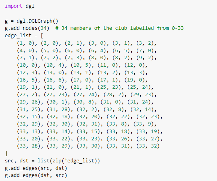
In the above dataset, there is no information on the members or the type of relationships between them, only the tie-ups based on whether they met outside the club. As you can see in the above code, the ‘edge_list’ contains edges from source nodes to destination nodes as well as from destination nodes to source nodes. This is because DGL internally uses a directional graph, and if we don’t make bi-directional connections, we will be introducing a directional relation that is not present in the original Karate club dataset.
We will label the first and last nodes representing the instructor and the administrator (0 and 33) as 0 and 1 respectively.
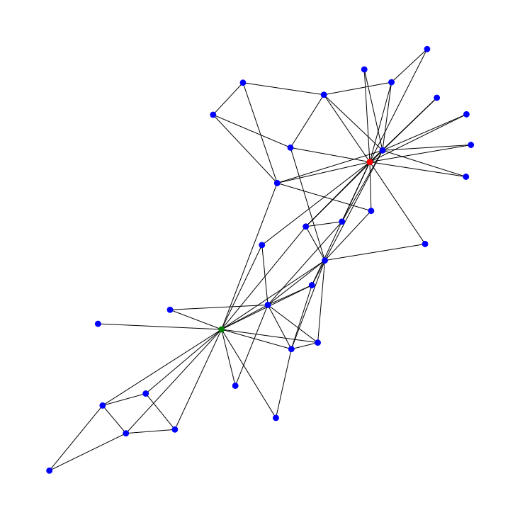
Now let’s visualize this DGL graph using the NetworkX library.
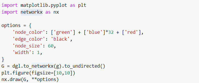
In the above code, we have given the colors green and red to the first and last nodes representing Mr.Hi and John A respectively. All the other nodes, unlabeled as of now, are given the color blue.
The output is shown below.
Defining the GNN Model
Now let’s create the GNN model in PyTorch. We will be using a custom Message Passing layer inside the model to solve our node classification problem. The MessagePassingLayer is defined below.
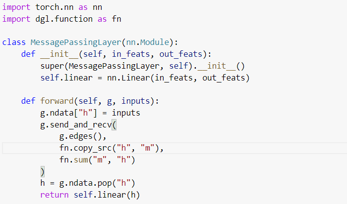
DGL provides a ‘send_and_recv’ method that will send messages along the given edges and update the embedding at the nodes. We have used ‘Sum’ as our aggregator function.
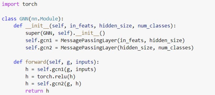
We will now create the GNN model with two MessagePassingLayers and a ReLu activation between these layers.
Training the GNN Model
Now let’s define the training hyperparameters and start training our model.
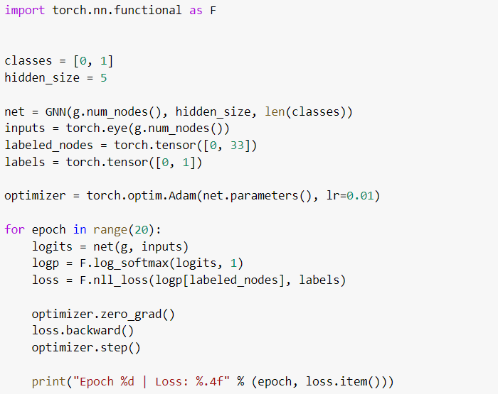
We have used a small hidden_size of 5 because we have a small graph to fit and increasing the number of trainable parameters might not be a good idea.
Our input to the model is an identity matrix of dimension 34x34 representing the initial condition that each member is not part of any group. We are going to use the Negative Log Likelihood loss function on the Softmax layer outputs of the first and last nodes because we only know the ground truths of these two nodes. For all the other nodes, this setting works as a semi-supervised learning mechanism.
Each message passing layer does one hop of information passing. That means, in the first message passing layer, each node embedding gets updated with information about its neighbors and in the second message passing layer, each node embedding gets updated with information on the neighbors of its neighbors. In the final softmax layer, we classify all the nodes and backpropagate the loss. The model will learn to update the node embeddings of each node based on its neighborhood and label them as 0 or 1 based on this embedding.
Evaluating the GNN Model
In the evaluation stage, the message passing layers calculate the node embeddings and the final softmax layer classifies each node as 0 or 1.
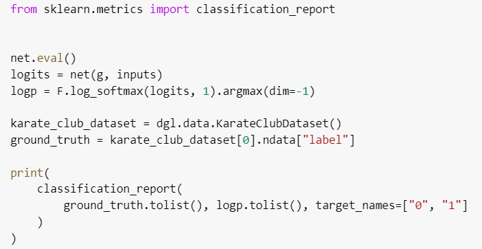
We will be using the ground truth from DGL’s KarateClubDataset class to evaluate the result. The classification report of our evaluation is given below.
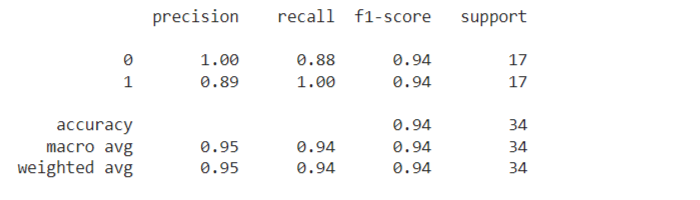
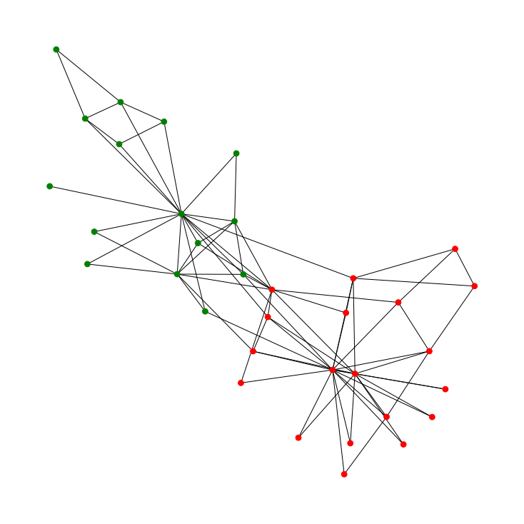
We were able to achieve 94% accuracy in under 20 epochs of training. The predicted graph is shown below.
You can access the full code here.
Conclusion
The Graph Neural Network is a powerful tool that can learn complex relationships within a dataset. Even though there is a higher effort in creating a dataset and defining the model for a Graph Neural Network, the complex information it can learn makes it a good candidate for solving problems that involve learning from not only the data points but also the relationships between them.