Price Elasticity 2.0: From Theory to The Real World

Executive Summary

Old Adages

As the once famous adage goes, “The most famous law in economics, and the one economists are most sure of, is the law of demand“—a law which states that the quantity of a given good purchased has an inverse relationship to its price—i.e., higher prices lead to lower quantities demanded, and that lower prices lead to higher quantities demanded. It is upon this premise that the entire discipline of microeconomics was built.

The relative responsiveness of the change in quantity demanded (Q) to any given change in unit price (P) is what is known as the price elasticity of demand, also referred to as PED or price elasticity. This article will introduce the fundamentals of price elasticity theory in somewhat lecture style before forcing us out of the classroom and into an exploration of real-world application, including pricing and promotion strategy design, how elements of behavioral and consumer psychology complicate the pristineness of the Nobel-winning theory, and a live case using Uber’s surge pricing model as the perfect application of price elasticity of demand.

But first, let’s begin with the basics. To deeply understand what price elasticity of demand measures, I must take you back to the beginning—to economics’ first principles—and help you understand the core concept of demand.

Economics 101: Understanding Demand

At its most elemental, demand is the quantity of a given good that a consumer is willing and able to purchase at every price along a continuum. Both theoretical economists and business people alike represent and measure demand using the demand curve, which is formally defined as the graphical representation of the relationship between price and the quantity demanded at any given point in time.

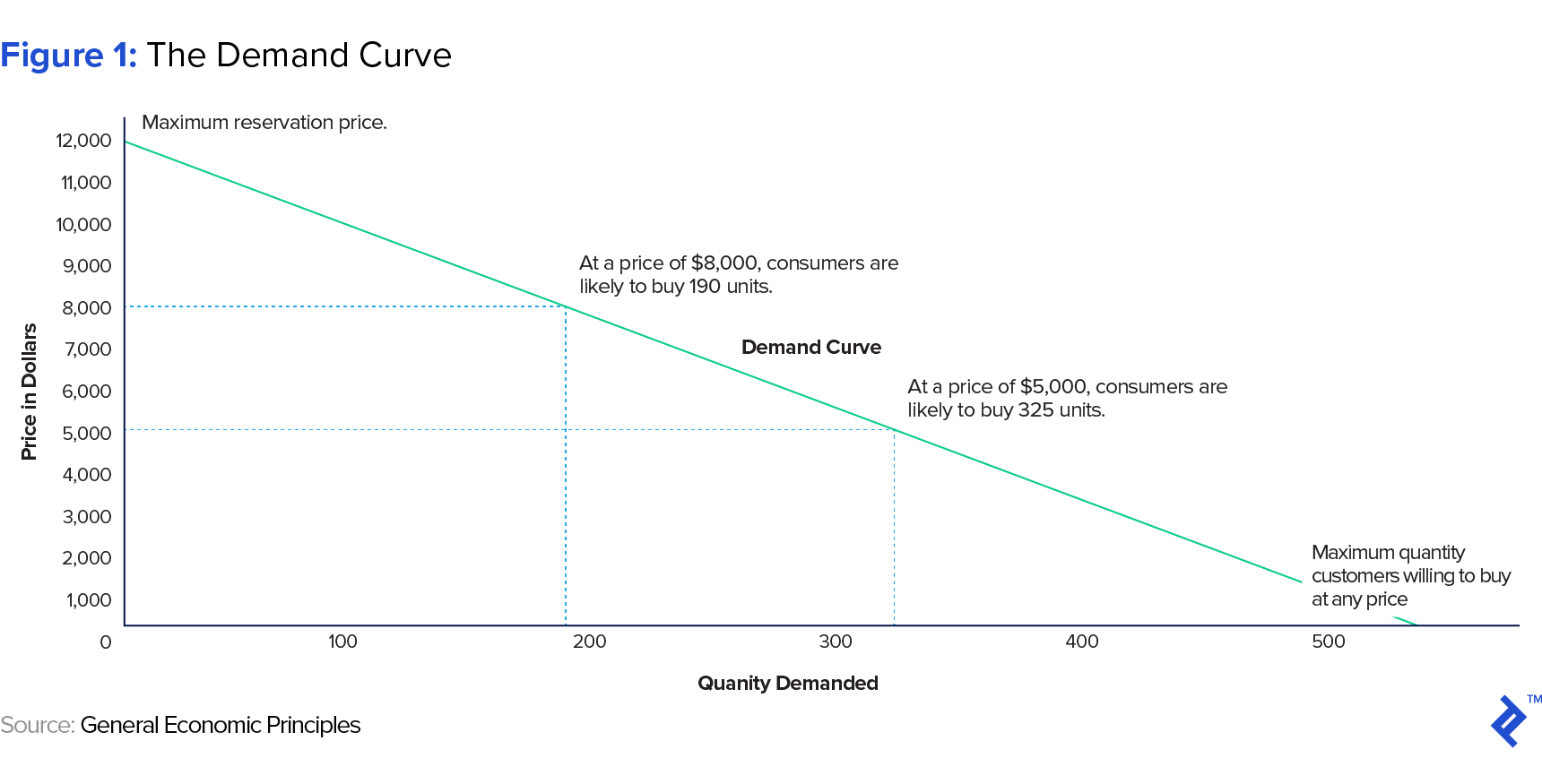
In a typical representation (such as the one illustrated in Figure 1 above), the demand curve is drawn with price on the vertical (y) axis and quantity on the horizontal (x) axis, with the function plotted (the curve) conventionally reflecting a negative association—i.e., a downward slope—that migrates from left to right.

Analyzing a typical representation further, the point at which the demand curve crosses the y-axis captures the price at which a customer will purchase zero units of given product because it is officially too expensive. This indicates the outer bound of a customer’s willingness to pay. Conversely, the point at which the demand curve crosses the x-axis captures the maximum quantity a customer is willing to buy at any price. Or framed differently, the maximum number of units a given firm can sell assuming it prices its product at zero.

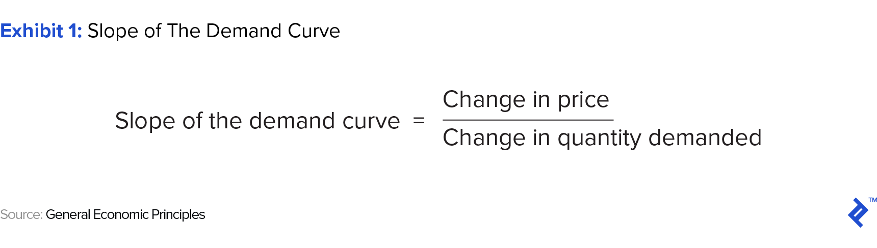
The demand curve is linear in its most basic form and its slope represents the probable purchase quantities at various prices, calculable using the following formula:

With the abstract concept of demand introduced, we must next understand the major law and associated factors that govern it.

The Law of Demand

The law of demand states that, ceteris paribus, the quantity demanded of a given good has an inverse relationship to its price—in other words, that higher prices lead to lower quantities demanded, and lower prices lead to higher quantities demanded. Excluding price, there are five other factors that conventionally govern demand elasticity. They are as follows:

1. Price of related goods. Related goods come in the form of either complements; i.e., goods with a positive cross-elasticity of demand, and thus typically consumed together (think, cars and petrol), or substitutes; i.e., goods with a negative cross-elasticity of demand, which are thus easily substitutable for one another (e.g., bottled vs. tap water). Specifically to the point, a rise in the price of a complement typically induces a rise in the overall cost of the bundle of goods, and thus a fall in the quantities demanded of both. Whereas with substitutes, the opposite effect takes place.
2. Income of buyers. When the income of an individual or the aggregate rises, individual and aggregate demand rises in line with the product’s marginal utility function. Marginal utility, in this case, is defined as the additional unit of satisfaction a consumer gains from consuming one more unit of a given good; utility which typically diminishes over time and/or with each additional unit consumed.
3. Tastes or preferences of consumers. Positive changes in the tastes or preferences in favor of a good (or brand within a good-category), naturally increases demand, and vice versa. It is for this reason that billions of dollars are spent annually on branding, advertising, and marketing in an effort to shift or manipulate tastes, preferences, and the stickiness of customers in favor of a given firm’s product/brand.
4. Consumer Expectations. Intrinsic to this variable are two other cornerstone economic principles. The first is the concept of future value, and the second, the concept of discounting to present value. Explained simply, when consumers expect that the value of a given product will rise in the future, there will be a higher willingness to pay for it in the present, thereby inducing greater demand. This concept exists at the nexus of where even basic consumer discretionary goods can begin to be considered investments solely on the basis of perception, consumer psychology, and fashions/trends.
5. Number of buyers in the marketplace. Simply put, holding income per capita constant, a rise in the aggregate number of addressable consumers, either due to demographic shifts or improvements in product relevance, will induce greater demand. The more people exist to consume a product that is relevant, affordable, and accessible, the higher overall demand, and vice versa.

The Demand Curve Revisited: A Shift in… vs. A Movement along…

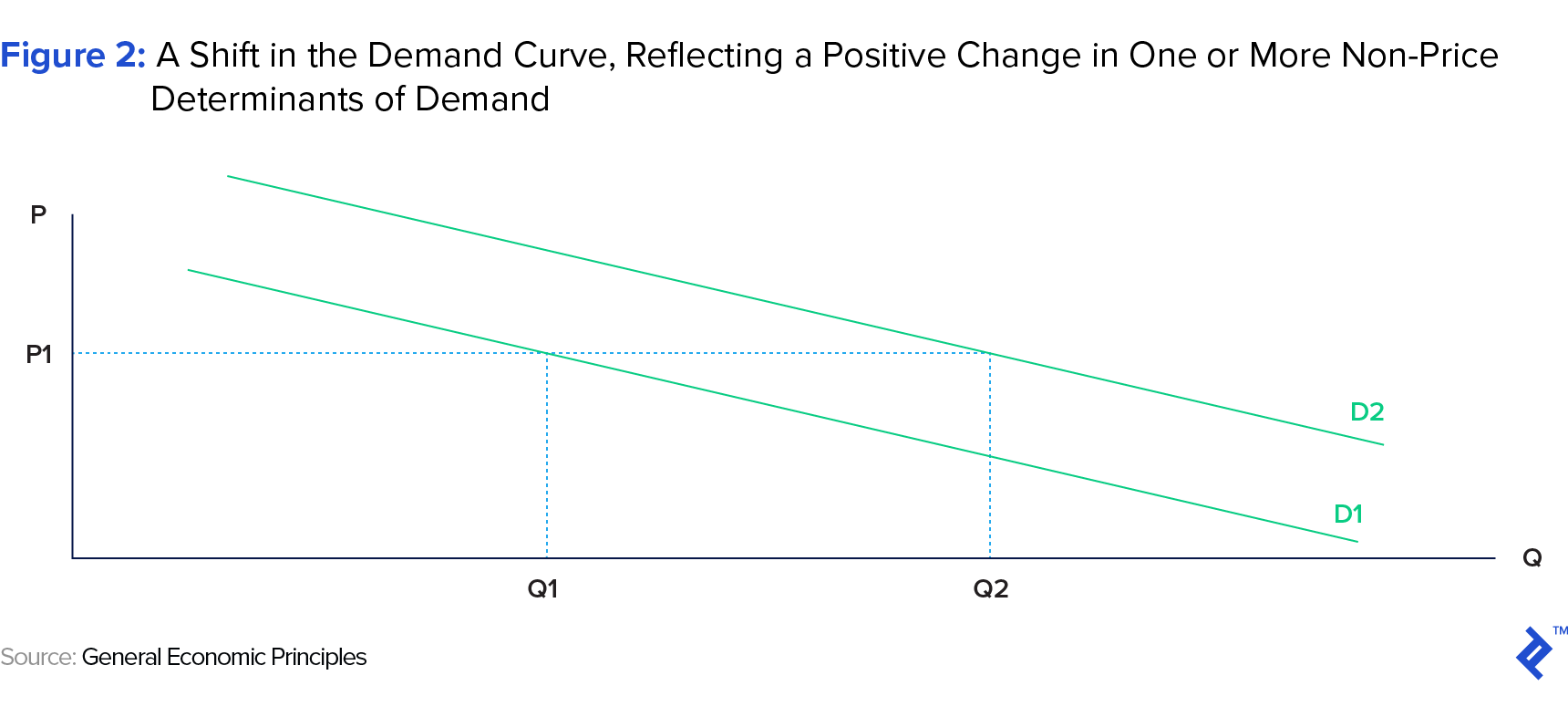
At this juncture, it is worth highlighting that, in economics, two different expressions of change in demand exist. The first is exemplified by a shift in the demand curve and the second by a movement along it. A shift in the curve can only be induced by changes in one of the five non-price determinants of demand, as detailed above and illustrated below in Figure 2.

A movement along the demand curve, on the other hand, only takes place in response to price changes, inducing a change in quantities demanded but within the bounds of the demand function/curve. Again, the sensitivity of the change in quantity demanded to the change in the elected price is what is known as the price elasticity of demand and what we will delve into next.

Price Elasticity of Demand

The price elasticity of demand (PED) measures the percentage change in quantity demanded by consumers as a result of a percentage change in price. This measurement of price elasticity of demand is calculated by dividing the % change in quantity demanded by the % change in price, represented in the PED ratio.

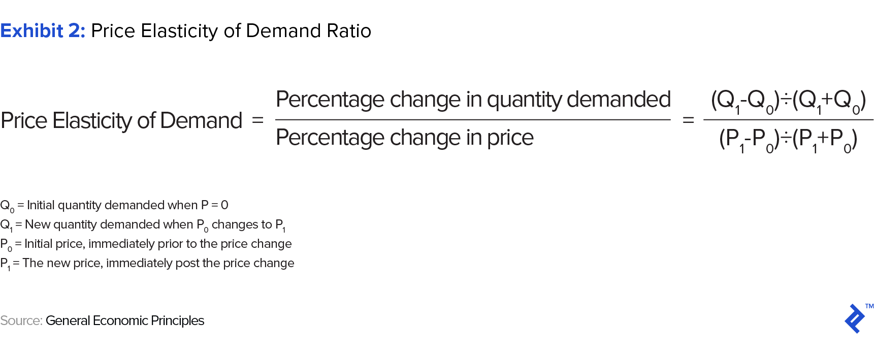
The elasticity coefficient—i.e., the output of the price elasticity formula—is almost always negative due to the inverse relationship between quantity demanded and price (the law of demand). It is worth noting, however, that the negative sign is traditionally ignored, as the magnitude of the number is typically the sole focus of the analysis.

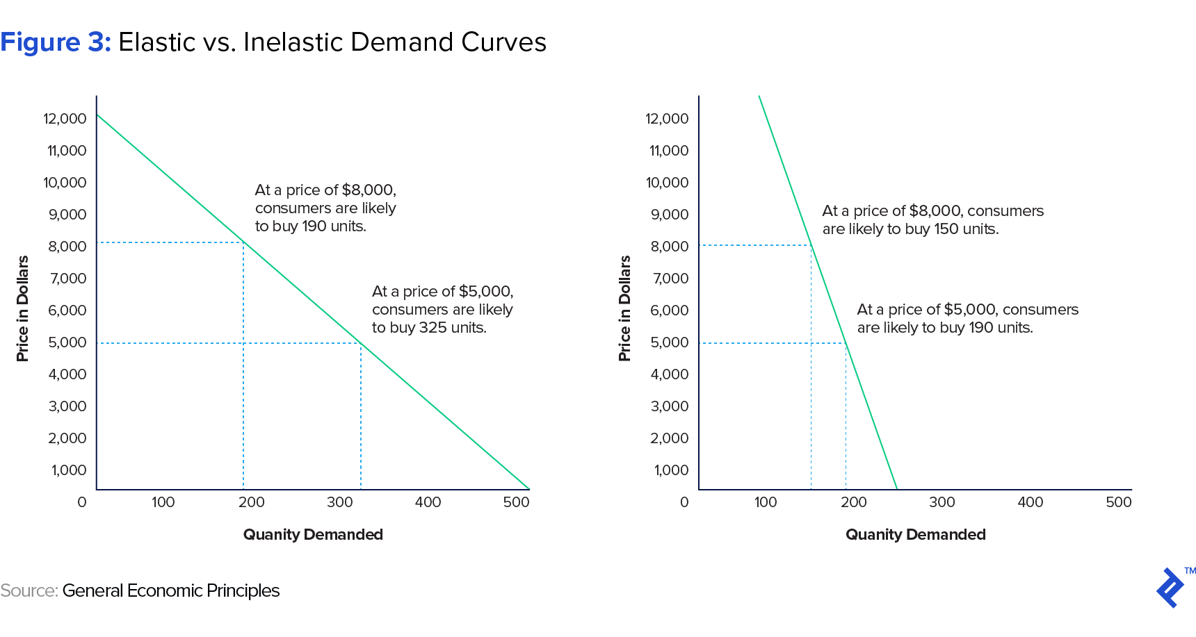
Interpreting Elasticities

Demand is considered elastic when a relatively small change in price is accompanied by a disproportionately larger change in the quantity demanded, and demand is inelastic when a relatively large change in price is accompanied by a disproportionately smaller change in the quantity demanded. Outside of these extremities, unit elasticity refers to any scenario where a change in price is accompanied by an exact/proportional change in quantity demanded.

Mathematically, demand for a given product is considered relatively elastic when its elasticity coefficient is greater than one and is considered relatively inelastic when its coefficient is less than one. Finally, demand is said to be unit elastic when the PED coefficient is exactly one.

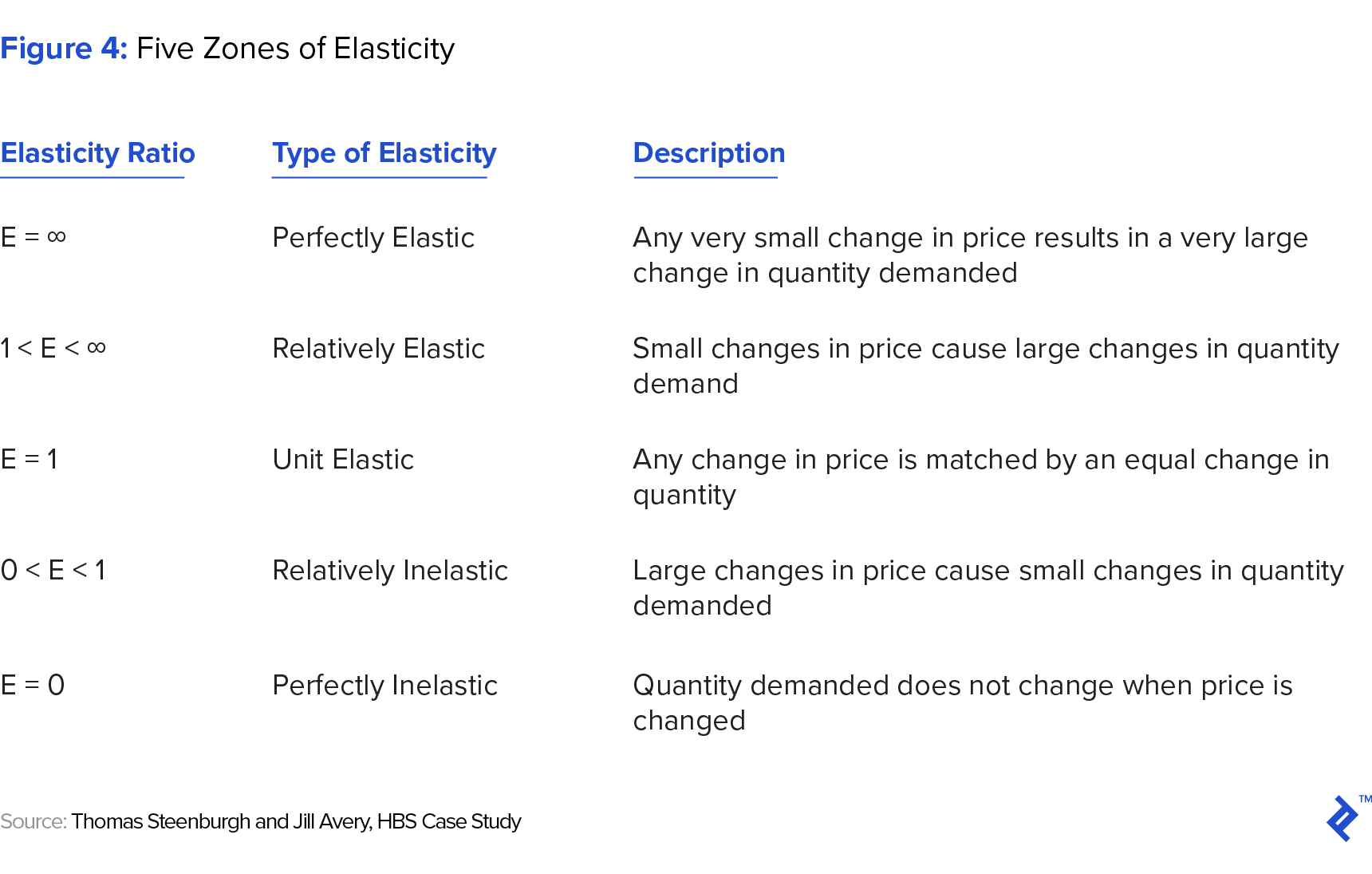
The Full Range of Elasticities

According to Thomas Steenburgh and Jill Avery, senior lecturers at the Darden School of Business and at Harvard Business School, there are five primary zones of elasticity:

How Do Companies Use Price Elasticity of Demand?

Switching gears somewhat, I would now like to explore the question of how companies use price elasticity of demand. To answer this effectively, we must again return to square one and redefine/clarify the function of a firm.

At its most fundamental, the function of a firm is twofold: (1) to create value for its customers, and (2) to capture value for its stakeholders. Businesses create value, or at least the perception of value, in their choice of what goods/services to produce and distribute; and capture value in the form of profits, in their choices of how to price and what cost structures to adopt. Thus, and more crudely put, it could be surmised that the core goal of a firm is to maximize profit.

With that settled, our next task is to understand the role of the marketer. We can probably all agree that their role, alongside other managers within a firm, is to further the goal of their firm, which we’ve defined as maximizing profit. And given that costs do not fall under the marketer’s purview, they must accomplish this by maximizing revenue. Adding a bit more structure to the conversation, a marketer does this by optimizing what classical business theorists refer to as The Four P’s: Product, Price, Place, and Promotion, where product describes the nature and relative differentiation of a good/service; price, what a good is sold for; place, where and how easily a good is accessed; and promotion, the marketing methods used to inform or persuade the target audience of a good’s merits.

Most specifically, it is the marketer’s job to estimate demand, anticipate the effect of various possible combinations of prices (price elasticities), and use that data to inform management on the most suitable pricing and promotion strategies for the firm and its products, assuming both product and place have been optimized.

The problem with price elasticity theory in the real world is that ceteris paribus can never hold; said differently, variables in competitive marketplaces can never be held constant. In reality, firms operate in dynamic, complex, and multivariate environments, replete with intangible competitive forces that interact with one another in impossible to predict/quantify ways. The real world, by definition, is imperfect, fluid, and inexact, not accounting for consumers.

A Brief Interlude: Price Elasticity and Behavioral Psychology

It is worth noting that the theory of price elasticity is a classical one and thus also ignores all the psychological, social, cognitive, and emotional factors that constitute people (which are typically accounted for in behavioral economics). Specifically, core to classical theories is the assumption that market participants are rational and thus always make the most normatively logical/optimal decision at hand. The reality is, and leaning on a recent and thoroughly insightful piece by Toptal Expert Melissa Lin, 80% of economic agents deviate from the objectively rational choice due to cognitive and emotional biases that influence how they process and act on information. This is a timely subtopic, given that Richard Thaler, Professor at the University of Chicago, was awarded the 2017 Nobel Prize in Economic Sciences for his work in behavioral economics.

A Real Life Case Study: Uber and the Phenomenon of Surge Pricing

Uber exists as a fantastic real-life case study of both price elasticity in action and how behavioral factors often influence expected outcomes. Specifically, its once contentious surge pricing feature is one that uses vast troves of data on supply (of drivers) and demand (by riders) to regulate prices in real time and maintain equilibrium moment to moment.

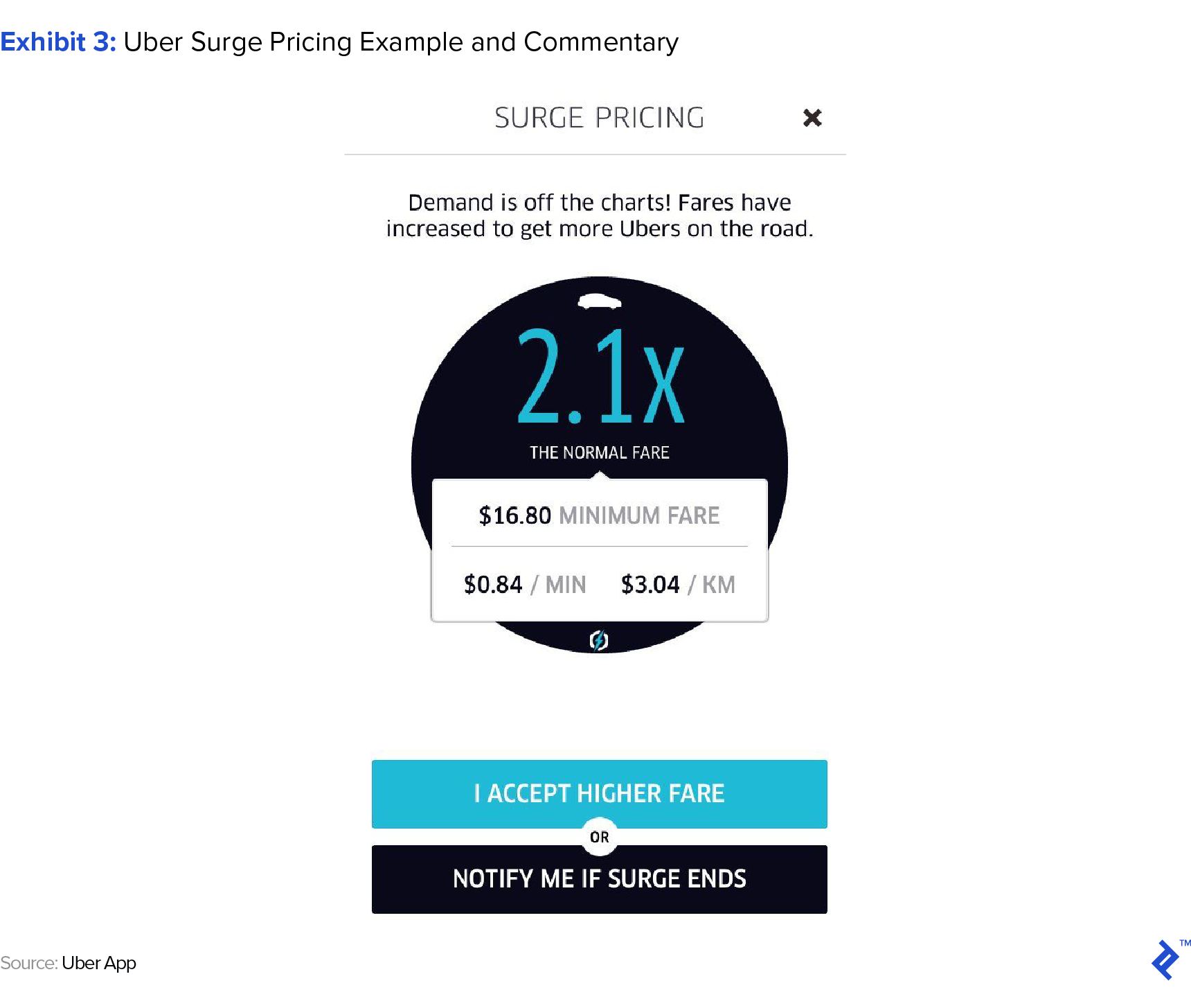
Note: What the cheeky comment doesn’t say but is artfully communicating is: “Demand is off the charts! Fares have increased to get more consumers off the app.”

Uber, given the sheer volume of real-time data it has available to it, is able to continuously triangulate its price elasticity quotient and use that information to regulate demand, moment-to-moment, which it does by pricing out different cohorts of customers who exist along its price sensitivity spectrum. Paraphrasing Keith Chen, a UCLA behavioral economist and Uber’s head of economic research: Just as conventional economics would predict, surging the price dampens demand. Specifically, and speaking to the early days of surge, when you would go from none to a 1.2x surge, you would see a consistently precise 27% drop in demand. Applying figures to theory, this implies a price elasticity quotient of 1.35, assuming a reasonably consistent baseline fare within the geographic bounds of the case, and a conclusion that Uber’s customers are relatively price elastic.

Things begin to get a bit more interesting when behavioral psychology comes into play. In Uber’s case, Chen goes on to explain that a strong round number effect, where pricing is concerned, seems to be at play with Uber’s consumers. Specifically, when Uber would go from 1.9x to 2.0x surge, one would observe a six times larger drop in demand than in going from 1.8x to 1.9x surge. Further analysis revealed that the 2.0x number just felt viscerally larger and thus “capricious and unfair.”

Even more interestingly, it turned out that when the surge multiplier moved from 2.0x to 2.1x, people actually took more rides. But it wasn’t that that customers preferred to pay 2.1x than double the rate, but because they assumed that if the price of the trip had been set at 2.1x, there must be a smart algorithm in the background at work and thus, it didn’t seem quite as unfair. Classic cognitive dissonance at play.

Uber as a case study perfectly encapsulates the challenge of applying theoretical price elasticity theory to real-world multivariate environments. Even science, it turns out, is more art than science, at least in the real world.

Subliminal Messaging: Other Applications of Price Elasticity of Demand

In addition to being used as an active/predictive tool, price elasticity also has other applications. Specifically, it is often used as a lag indicator, used to inform on how companies are performing across a range of parameters. These parameters include product performance, branding/marketing performance, competitor and complement performance, and even overall macroeconomic health.

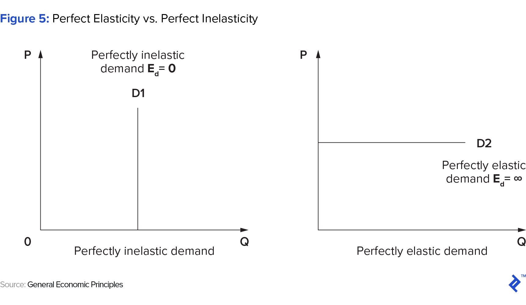
Product. Paraphrasing Jill Avery, Senior Lecturer at Harvard Business School, all companies seek to create products and services that offer unique and sustainable value to their customers, especially relative to marketplace substitutes. Referring briefly to Figure 5, the more unique/differentiated a given product, the higher the customers’ willingness to pay on the same total cost basis, and the more inelastic its demand will be. Price elasticity of demand is thus an effective indicator of both true or perceived product differentiation within a market.

Branding/Marketing. Related to this is the distinction between true and perceived product differentiation. True product differentiation aside for the moment, the perception alone of uniqueness, captured through the power of effective branding, is a powerful psychological determinant of success that must be harnessed by the marketer. Price elasticity thus serves as an effective lag measure of a firm/product’s brand equity in the marketplace relative to the competition. Where a product’s demand is relatively elastic, it is considered a commodity (i.e., weakly branded or undifferentiated and thus easily substitutable with the next best/lowest priced alternative) by consumers.

Competition and Complements. A company’s price elasticity of demand is also a great indicator for the state of both competitive intensity (i.e., the incidence of viable substitutes) and of complements in the marketplace. Relatively elastic price elasticities indicate either a highly competitive arena for goods at that price point or the fact that the cost/price of complements is on the rise.

Product/Business Lifecycle. According to Joel Deal, author of an HBR piece on new product pricing policies, price elasticity is also an accurate gauge of where your company is in its maturity; a concept he breaks down further into three distinct elements.

1. Technical Maturity: This is indicated by a declining rate of product development, increasing standardization or commoditization of features and performance among brands, and stabilization of customer expectations as a given product spends more time in the market.
2. Market Maturity: This form of maturity is indicated by consumer acceptance of a given product, its service idea, value proposition, and the stabilization of the belief that it will perform satisfactorily.
3. Competitive Maturity: This is indicated by the stabilization and entrenchment of existing players and brands, their market share, pricing, and positioning as a product continues to exist in the market.

State of Overall Economy. The final parameter which price elasticity of demand indirectly speaks to is the overall health of the economy in which a product is sold into. Specifically, this parameter relates to both demographics (i.e., the size of the addressable population) and the income levels of the constituents that populate that consumption market. Related to this is also the overall cost of the product being offered. Low income, high-cost product environments will naturally yield relatively elastic demand curves, while high income, low-cost products will yield relatively inelastic demand curves.

Looking forward…

Setting the right price for a given product is hard, and worse, has always been far from an exact science. Though the theory of price elasticity has been around for over a century, it has typically served as a theoretical framework to imprecisely understand market reactions to changes in price, the data from which would then be used to clumsily predict future behavior. It was a great start — we did our best with it and it certainly served its purpose.

But times are changing. The combination of big data’s proliferation and the rapid A/B testing possibilities purveyed by the digital economy are changing the precision and historical applicability of PED. Be it from Uber whose dynamic (surge) pricing feature helps it maintain supply-demand equilibrium in real time using price; to startups such as 100% Pure who have lifted operating profits by 13.5% over three months, companies are now able to predict with staggering accuracy not just by how much demand will change with every unit change in price, but also why—i.e., the psychology behind the swings.